
Most data sets which are readily available, have been cleaned for pedagogical purposes. In this post, we present a case study with a realistic touch. This simulated data set has 40,000 entries and 100 predictors, riddled with spelling mistakes, missing entries, etc to mimic real-life data faced by data scientists. This exercise will give us an opportunity to demonstrate a full stack approach towards data science. Success in this exercise hinges on feature engineering and minimize data leakage. The data set can be downloaded here.
EDA is an important first step towards understanding the data set. Here are four main reasons why:
- Error detection: It helps to check for NaNs, missing values, spelling mistakes, etc.
- Assumptions: Helps us understand the distribution of the predictors.
- Relationship between predictors: Assess the correlation of the different predictors.
- Model selection: Enables a proper model to be chosen.
Read the data set
First, we will read the data (train.csv) using pandas, and store the indices of the numeric and categorical predictors separately. This will be important in later analyses, since different EDA techniques are used for numeric and categorical predictors.
import numpy as np
import pandas as pd

# Read csv file
df = pd.read_csv('train.csv')

# Store indices of numeric predictors
num_index = np.array(df.select_dtypes(include=['float']).columns)

# Store indices of categorical predictors
cat_index = np.array(df.select_dtypes(include=['object']).columns)
Univariate EDA
We print out general descriptive statistics using df.describe() which gives the user a brief summary of the predictors. For numeric predictors, count, mean, std, min, max as well as lower, 50 and upper percentiles, will be provided. For categorical predictors, count, unique, top, and freq will be given, where top is the most common value and freq is the most common value’s frequency.
A graphical means is well suited for a quick overview of the distribution of the predictors. We use seaborn for this purpose and apply the following lines of code.
import seaborn as sns

ax = sns.boxplot(x=df[num_index])
It is important to note that we are only able to use boxplots for numeric predictors, and that’s when the stored indices for numeric predictors comes in handy.
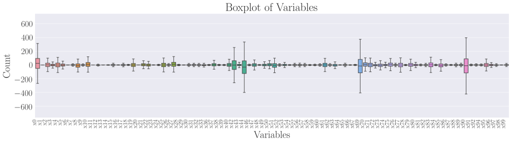
Click the image to have an enlarged view of the plot. We observe that outliers were present approximately symmetrically (at both the high and low ends of their respective distributions) in a few predictors, such as x0, x44, x70 and x91. This will be critical in model selection later on, as some models (e.g. CART models) are more resistant to outliers than traditional regression models.
For categorical predictors, we use seaborn’s countplot to plot out the frequencies of each unique value in the predictor. The function to call is as follows,
for i in range(len(cat_index)):
    sns.countplot(data=df, x=cat_index[i])
The cat_index array contains the previously stored indices to identify categorical predictors. The code loops over all categorical predictors and plots a countplot for each of them. Using predictor x35 as an example, we see that there exist spelling errors such as wednesday and wed, thursday and thur, friday and fri. The model will lose valuable data and hence predictive power, if such errors are left unchecked.
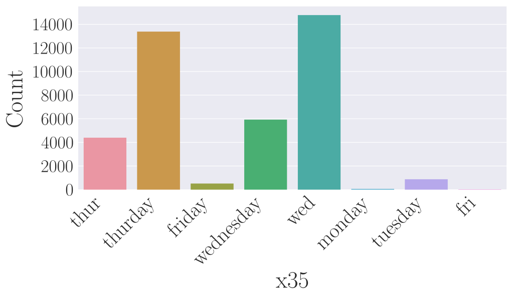
x35.Bivariate EDA
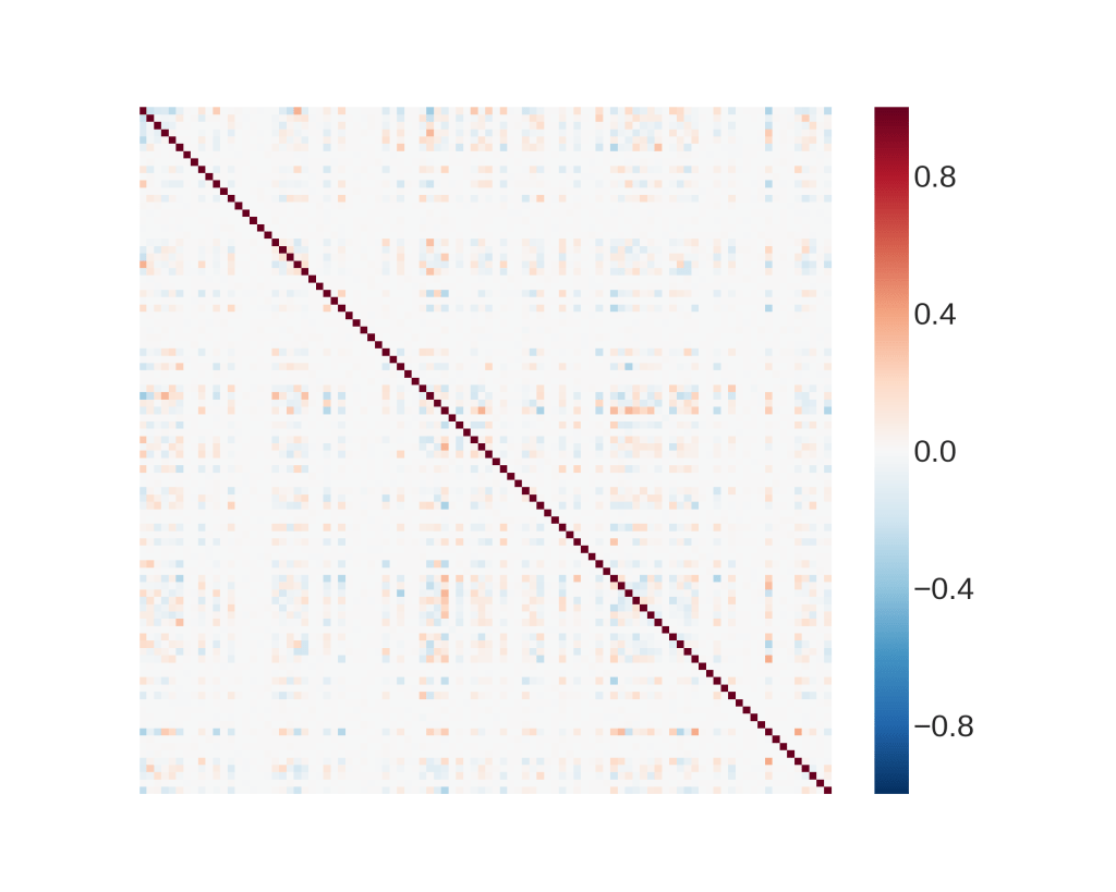
Bivariate methods look at two predictors at the same time, to determine their relationship, if any. Such analyses give us valuable information about the correlation between any two predictors, and preventative measures can be taken to tackle potential problems such as multicollinearity. As usual, categorical and numeric predictors have different methods for bivariate analysis. We first look at numeric predictors using the Pearson correlation heatmap. It is a quick graphical method to observe correlation between any two numeric predictors. The code is shown below.
# EDA for numeric predictors - Pearson correlation heatmap
corr = df[num_index].corr(method='pearson')
sns.heatmap(corr, xticklabels=corr.columns, yticklabels=corr.columns)
The resulting plot shows that there is no significant correlation between any two predictors. This can be tricky for the model selection since the predictors appear to behave like random numbers.
As for categorical predictors, we use cross-tabulation to analyze the data. Cross-tabulation is one of the basic non-graphical bivariate EDA methods for categorical data, and it allows us to see the relationship between any two predictors. Over here, we are interested to observe the relationship between each categorical predictor x and the outcome y. Using x35 as an example, we achieve this by writing the following code.
# EDA for categorical predictors - cross-tabs with outcome
for i in range(len(cat_index)):
    print(pd.crosstab(df[cat_index[i]], df.y))
The output shows a cross-tabulation between the various categories in x35 against the outcome y.
| y | 0 | 1 |
| x35 | ||
| fri | 19 | 7 |
| friday | 436 | 85 |
| monday | 38 | 28 |
| thur | 3676 | 729 |
| thurday | 11029 | 2349 |
| tuesday | 582 | 300 |
| wed | 11702 | 3073 |
| wednesday | 4422 | 1516 |
x35 and outcome y.Looking at this cross-tabulation, we can already observe that most of the predictors result in the outcome 0 and fewer in 1. This is a fair warning and in fact, a simple analysis on the outcome will show that approximately 80% of the data has an outcome of 0 and 20% of them has outcome 1. As such, this data is slightly imbalanced, and some care is needed in order for the machine learning model to be able to pick up the minority outcome of 1.
