
This article discusses the most commonly used performance metrics in classification and regression machine learning problems, in the hope that users will be familiarized with how the metrics are calculated, what the calculated metrics mean, and when is that metric useful. It is critical to understand that no single metric can validate the result entirely. Each one shows a different side of the story, and together they provide a well-validated performance evaluation of the machine learning model.
Classification Metrics
Over here, we introduce some of the most commonly used metrics for classification problems, and discuss the side of the story each metric presents.
Classification Accuracy
The classification accuracy is measured as the proportion of correctly classified events out of all events.

This is a straightforward accuracy metric which makes much sense at first, but proves itself to be too naive in reality. For example, in a data set with 99 actual positive events out of a 100, if the model is totally erroneous and predicts all events to be positive, it will attain a classification accuracy of 0.99. This number is deceivingly high, only because the data set is imbalanced.
- Pros: Simple, and straightforward calculation.
- Cons: Provides true insights only if data set is balanced (i.e. 50% positive, 50% negative). It is simply not useful as a metric in most scenarios to evaluate the true predictive power of a machine learning model.
Confusion Matrix (not a metric, but very important)
We start off with a validation technique so important that it cannot be neglected. The confusion matrix is a vital step in the validation process because it shows concisely in one matrix, the simulated results of your model. All diagonal blocks in the confusion matrix are correctly classified cases, while the off-diagonal blocks represent the mis-classified cases by the model.
| Predicted | |||
| Positive | Negative | ||
| Actual | Positive | True positive | False negative |
| Negative | False positive | True negative |
- True positive: This refers all cases that are correctly predicted to have the positive condition.
- True negative: This refers to all cases that are correctly predicted to have the negative condition.
- False positive: The false positive condition refers to cases where the model classifies the data to be positive, when the actual classification is negative. This is more popularly known as the false alarm and is termed Type I error by statisticians. False positives are deemed more adverse in some justice systems, which believe that it is better for 10 guilty men to get acquitted than for an innocent man to suffer.
- False negative: Similarly, the false negative condition refers to cases where the model classifies the data to be negative, when the actual classification is positive. This is also known as Type II error. False negatives are critical in cases such as cancer classification, where it’s absolutely important that all cases of malignant cases are identified. Even a single case of false negative in this instance could lead to dire consequences.
Over- or under-prediction due to poor modeling techniques on imbalanced data sets will show up very sharply on the confusion matrix, due to very small numbers in one of the cells. The confusion matrix, although not a “metric”, is introduced because many useful metrics are derived from it. We continue with the list, with the terminology introduced in this section.
Precision
Precision is calculated as follows.

The sum of all predicted positive condition refers to the sum of true positives and false positives. This metric is a number that ranges [0, 1] where 1 is the best result. It retrieves all its information from a single column of the confusion matrix and there are certain pros and cons to what this metric tells us.
- Pros: Informs the accuracy of the model better than using the classification accuracy, since it includes false positive predictions in its calculations.
- Cons: Might not be able to validate the model in a more well-rounded manner since it does not use information from predicted or actual negative conditions. In a previous article, we showed that the precision metric was unable to tell that the model was in fact over-predicting the majority outcome in an imbalanced data set.
Recall / Sensitivity / True Positive Rate (TPR)
Recall is another metric that can be derived from the confusion matrix and is calculated as follows.

The denominator, which is the sum of all actual positive conditions refers to the sum of true positives and false negatives. This is also a metric which ranges between [0, 1], with 1 being the most optimal. This metric retrieves all its information from a single row of the confusion matrix. By doing so, it validates the model from a different view.
- Pros: Will be very useful for models predicting imbalanced data sets, since the false negatives are included in its computations. Over-prediction of majority outcomes in an imbalanced data set (which is undesirable) will be picked up.
- Cons: Might not be a good metric to determine the model’s predictive power for a single outcome (either positive or negative), if the user is only interested in having high predictive power in predicting one of the outcomes.
Specificity is sometimes mentioned as a separate metric, but it should really be thought of as recall applied to the negative class. In other words, specificity should not be thought of as a different metric, but simply applying recall to a different class, in a multi-class classification problem. That is why in scikit-learn, the classification_report provides precision, recall, and f1-score for each of the classes separately.
F1-score (Harmonic Mean)
Unfortunately, precision and recall are often in a tug-of-war, such that high precision leads to lower recall, and vice versa. Precision measures the percentage of cases classified positive, whereas recall measures the percentage of actual positive cases that were correctly classified. Increasing the classification threshold decreases false positives and increases false negatives, and in turn precision increases and recall decreases. As such, both metrics must be examined at the same time, and we wish for some kind of middle ground, where both recall and precision are simultaneously close to 1. As such, the f1_score calculates the harmonic mean between recall and precision, allowing the user to have a more well-rounded metric. The f1-score is a metric which ranges between [0, 1] where 1 is the most optimal.

- Pros: A metric which simultaneously involves recall and precision, giving equal importance to both metrics.
- Cons: In real-life scenarios, the cost incurred by mis-classifications are different in different scenarios. In other words, sometimes the cost of false negatives can be costlier than false positives. As such, weighing recall and precision with respect to this associated cost would be prudent.
Fowlkes-Mallows Index (Geometric Mean)
Previously, we have seen a harmonic mean between recall and precision. An arithmetic mean refers to the mean of sums, harmonic mean refers to mean of reciprocals, and geometric mean refers to mean of multiplications. The various types of means show the different sides of the model’s performance and tells us a fuller story, with regards to its predictive power. The sklearn.metrics.fowlkes_mallows_score is defined in scikit-learn as the geometric mean between recall and precision.

- Pros: The Fowlkes-Mallows index ranges between [0, 1] and measures the similarity between two clusterings. The higher the index the more similar the clusters. In this case, we do hope for a higher geometric mean since we would like the recall and precision to be simultaneously high in value. This index has also been proven to be resistant to noisy data sets.
- Cons: Similar to the f1-score, realistic weighting associated to cost of false negatives and false positives can tailor the metric better for specific scenarios.
Receiver Operating Characteristic (ROC) curve
The ROC curve plots the curve of True Positive Rate (TPR) against False Positive Rate (FPR) under various threshold settings. Threshold settings determine when a certain data will be classified as positive. Such a metric is useful for machine learning models that calculate probabilities for classifying data, e.g. logistic regression. False positive rates are simply 1 – specificity, and true positive rates are recall (where the formula is given above). An example of a ROC curve is shown below.
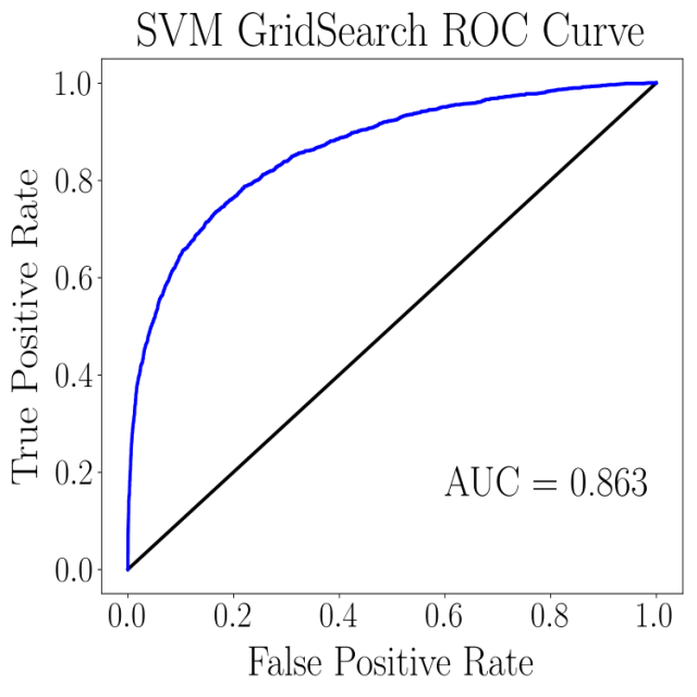
The top left hand corner (0, 1) gives the perfect classification where there is 100% recall (no false negatives) and 100% specificity (no false positives). As such, a ROC curve that stretches as far out to the left hand corner as possible would be deemed most optimal. The diagonal line is drawn to show the ROC curve of a completely random classification. Any machine learning model should do better (and hence be plotted above this no-discrimination line) than a random guess.
- Pros: Provides a good visualization to gauge overall performance of model and pick a good threshold setting for the model.
- Cons: Will not be able to reveal common problems in imbalanced data sets, such as over-prediction of majority outcomes. Summarizing metrics, as such, tend to be overly-optimistic.
Area under curve (AUC)
The AUC score is simply the area under the ROC curve as shown above. As previously mentioned, the ideal curve would stretch as far out to the top left hand corner (0, 1) as possible, and hence the AUC score is a metric ranging between [0, 1], with 1 being perfect. In fact, the AUC score should not be lower than 0.5, since that would imply that the machine learning model is worse at classifying the data set than a random guess.
- Pros: Simple metric that quantitatively tells the user how well the ROC curve looks.
- Cons: It ignores the predicted probability values, and summarizes performance in regions of the ROC curve where the model rarely operates.
Regression Metrics
Metrics for regression problems are different from those of their classification counterparts, because the predicted values are numeric and continuous. Regression, typically, involves fitting a best-fit line/curve to a set of training data. The predicted values would differ from the actual values, and hence metrics exist to measure this difference and give an evaluation of the model’s predictive power.
Mean Squared Error (MSE)
The mean squared error measures the sum of the squared errors and takes an arithmetic average.

This metric is a measure of the quality of the model’s predictive power, and values which are closer to zero are desirable. Sometimes, the square root of the MSE (RMSE) is taken to measure the deviation of the predicted values from the actual values.
- Pros: Straightforward metric for summarizing the quality of the model as a whole.
- Cons: MSE gives too much attention to outliers, because outliers give larger errors from the squared term. Models which tune their parameters using the MSE results in higher final error due to heavier weight given by outlier errors.
Mean Absolute Error (MAE)
A variant of the MSE is the MAE which computes the arithmetic mean of sum of the errors, without squaring it. This gives an error measurement which is more robust to outliers.

- Pros: Robust to outliers.
- Cons: May not be suitable for scenarios where the user would like the model parameters to penalize the outliers more heavily.
R2 (R Squared)
The R2 value is also known as the coefficient of determination. This coefficient ranges from [0, 1], with the most optimal value as 1. The most common definition of R2 is as follows.

where

and

R2 can be explained in a number of ways, but it is most intuitive and common to illustrate it in terms of explained variance. For example, if the R2 value of the resulting model is 0.82. Then, one can say that 82% of the variability of the dependent variable has been accounted for, while the remaining 18% is unaccounted for. In statistics, if the R2 value is 1, it is a perfect fit. However, in machine learning, a perfect fit to the training data implies over-fitting. This is a bit of a conundrum, where we would like the R2 value to be as close to 1 as possible, without over-fitting.
- Pros: A good way to assess the goodness-of-fit of a regression model.
- Cons: R2 values are not as straightforward to understand by themselves. They work best when used in conjunction with residual plots, and other statistical metrics. Some data sets inherently have a greater amount of unexplained variance, and small R2 value does not imply that the model is poorly fitted. Even with low R2 values, important conclusions can still be drawn from the model if the independent variables are statistically significant.
