Time series analysis is of great importance in quantitative financial analysis where the ability to accurately forecast stock prices using past stock prices allows investment companies to know when to buy, sell, or hold on to stocks. In today’s article, we will explain and demonstrate with real world financial data, attempting to forecast the open stock price for NASDAQ: AMZN (Amazon.com, Inc.).

Traditional statistical methods such as Auto Regressive Integrated Moving Average (ARIMA) models are an invaluable tool that has been used and applied extensively by quantitative analysts around the world. The ARIMA model consists of three main components.

1. AR (Autoregressive): The AR portion refers to the autoregressive model, where the evolving variable of interest is regressed with its own prior (lag) values.
2. MA (Moving-Average): The MA portion refers to the moving average model which indicates that the regression error is a linear combination of error terms at various times in the past.
3. I (Integrated): Integrated refers to the procedure of replacing values with a differencing of prior values. Such methods are sometimes necessary for transforming “non-stationary” data into “stationary”. Stationary data are stochastic processes that do not change when shifted in time. Parameters such as mean, variance stay the same over time.

ARIMA models are generally denoted by the notation ARIMA(p, d, q), where p is the order of the autoregressive model denoting the number of time lags, d is the degree of differencing where it refers to the number of past time values that has been used for differencing, and q is the order of the moving-average model. The ARIMA model is hence a generalization of a class of models, where ARIMA(1, 0, 0) would refer to an AR(1), ARIMA(0, 1, 0) would refer to an I(1), and ARIMA(0, 0, 1) would refer to an MA(1).

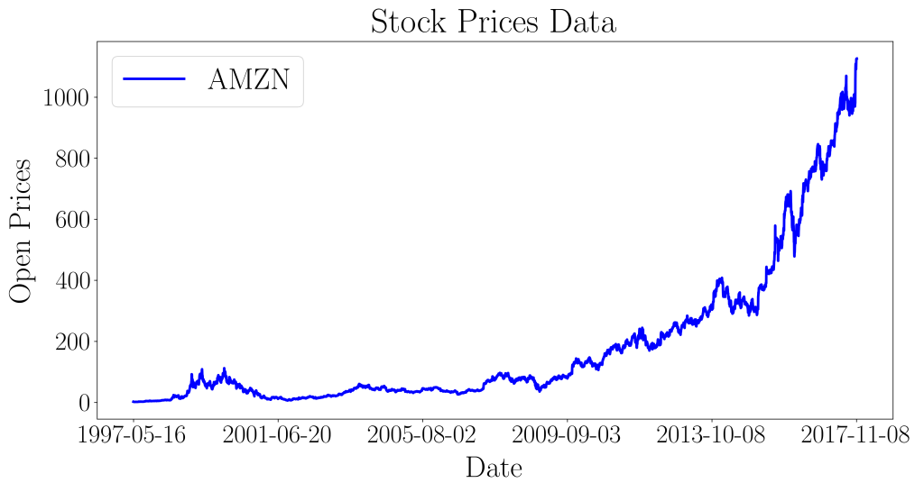
High quality financial datasets are usually not cheap, but fortunately we managed to find a great source on Kaggle. This data set contains full historical daily price and volume data for all US-based stocks and ETFs trading on the NYSE, NASDAQ, and NYSE MKT. We’ll be focusing on the Amazon dataset located at ‘Data/Stocks/amzn.us.txt’ in the downloaded folder. The financial data spans from 1997-05-16 to 2017-11-10.

The article will be split into the following sections:

1. Exploratory Data Analysis (EDA): Initial EDA will reveal the nature of the dataset, informing us of the proper parameters for the ARIMA model.
2. Data Manipulation: We’ll demonstrate how to split the dataset into 70% training data and 30% validation data. The validation dataset will be used for model accuracy validation.
3. Time Series Modeling: The ARIMA model will be used to forecast the remaining 30% (from 2011-09-22 to 2017-11-10). The forecast stock prices will be checked against the actual data from the validation set.

Exploratory Data Analysis

We first read the dataset as follows and only choose two columns: ‘Date’ and ‘Open’.

df = pd.read_csv('data/Data/Stocks/amzn.us.txt')[['Date','Open']]

This gives us the dates as well as the open prices at their respective dates. We go ahead and conduct standard EDA on the dataset. First, we plot the entire dataset to observe the trend of the prices.

Then, we plot the lag plot with the following code.

from pandas.plotting import lag_plot
lag_plot(df['Open'], lag=1)

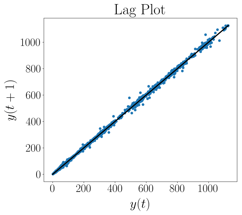
A lag plot tells us a few things: it shows us the presence of outliers (extremely high or low data values), randomness (data without a pattern), serial correlation (where error terms in a time series transfer from one time period to another), and seasonality (where fluctuations in data happen at regular time periods). Our lag plot reveals a linear shape, which suggests that an AR model is a suitable choice. As such, we will be setting q = 0.

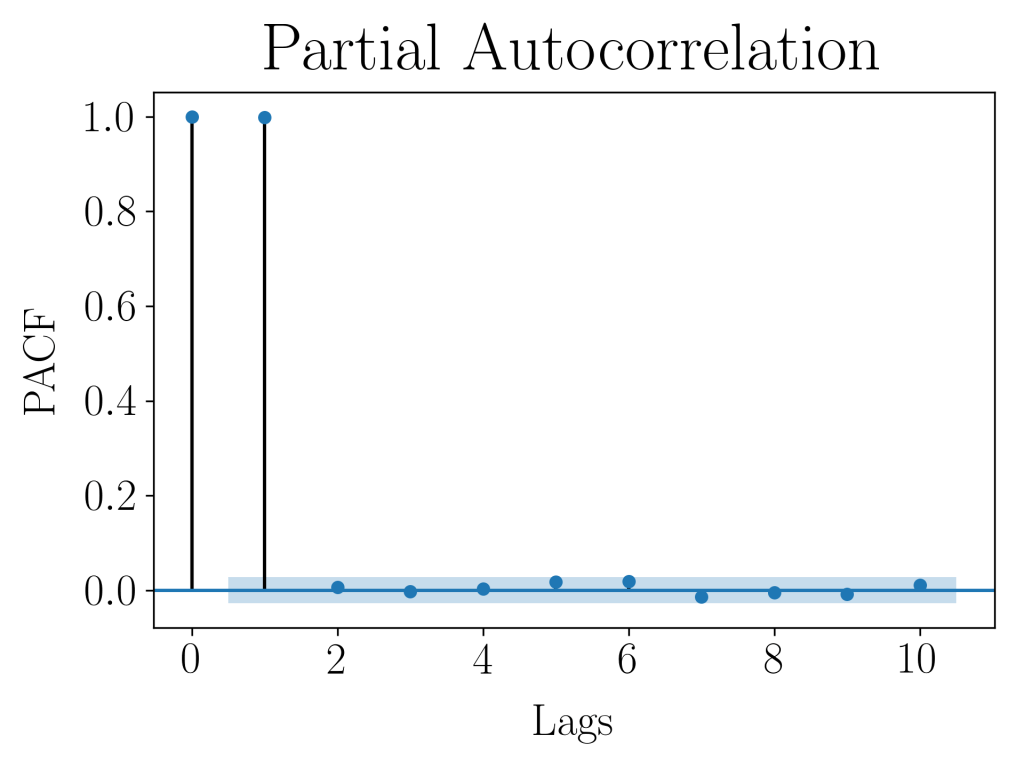
Next, we plot the partial autocorrelation function (PACF) values against time lags in order to figure out a suitable order for the AR model. PACF values tells us how significant adding another lag is when one already have x number of lags.

from statsmodels.graphics.tsaplots import plot_pacf
plot_pacf(df['Open'], alpha=0.05, lags=10)

The above code plots the PACF values against 10 time lags, and we observe that there is a significant positive lag-1 autocorrelation value, while the others are not significantly different from 0. This suggests the suitability of an AR(1) model for our dataset!

Data Manipulation

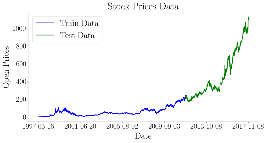
Now that we have decided on the parameters for our ARIMA model, we split the dataset into 70% train and 30% validation, in order to validate the accuracy of our model’s forecasting capabilities.

# Split dataset into 70% train, 30% test
train, test = df[0:int(len(df)*0.7)], df[int(len(df)*0.7):]

We plot the train and test set in the following graph, to clearly observe the trend of the stock prices, and the targeted forecast of the test set.

Time Series Modeling

The following procedure will be explained in detail, ensuring that both the concepts and the code, are easily understood and fully reproducible. First we assign the train and test set price values to y_train and y_test in the form of NumPy arrays. This will be necessary, as they will be used as inputs to other functions.

# Assign train and test set as numpy arrays
y_train = train['Open'].values
y_test = test['Open'].values

Next, we create new lists for the time series modeling process. hist will contain all historical data, and y_pred is a list of all predicted values. Right now, hist only contains the 70% train data and we will append new data to it as time progresses. y_pred is an empty list as of now, and we will also append new predicted values to it as time progresses.

# Create lists for updating new predictions
hist = [x for x in y_train]
y_pred = list()

We import the ARIMA model from statsmodels Python library, and the mean_squared_error function from Scikit-Learn. The recursive time loop might look overwhelming at first sight, so lets discuss the overall main objective of this time loop. At time t, we predict the corresponding price for time t+1. Subsequently, in the next time step (time t+1), when the actual price (y_test[t]) is now known, we append this into our list of training data hist, and use it to predict the price at t+2. All predicted values are appended into the list y_pred, and at the end of the time loop, we measure the normalized mean squared error of the forecast vs actual prices.

from statsmodels.tsa.arima_model import ARIMA
from sklearn.metrics import mean_squared_error

# Setting parameters for ARIMA model
p=1; d=1; q=0

# Recursive time loop for forecasting time series
for t in range(len(y_test)):
    # Instantiate ARIMA model
    model = ARIMA(hist, order=(p, d, q))

    # Fit model to the training set
    model_fit = model.fit(disp=0)

    # Forecast for next time step
    next_step = model_fit.forecast()

    # Append next step to prediction list
    y_pred.append(next_step[0])

    # Append new observation to training data
    hist.append(y_test[t])

# Calculate MSE
MSE = mean_squared_error(y_test[:-d], np.roll(y_pred, -d)[:-d])

An ARIMA model of ARIMA(1,1,0) sets the lag value to 1 for autoregression, uses a difference order of 1 to make the time series stationary, and uses a moving average model of 0. This time loop is known as a rolling forecast, and it is required given the dependence on observations in prior time steps for differencing and fitting the ARIMA model. For pedagogical purposes, we performed this rolling forecast by re-creating the ARIMA model after each new observation is received.

The stock prices forecast are as follows:

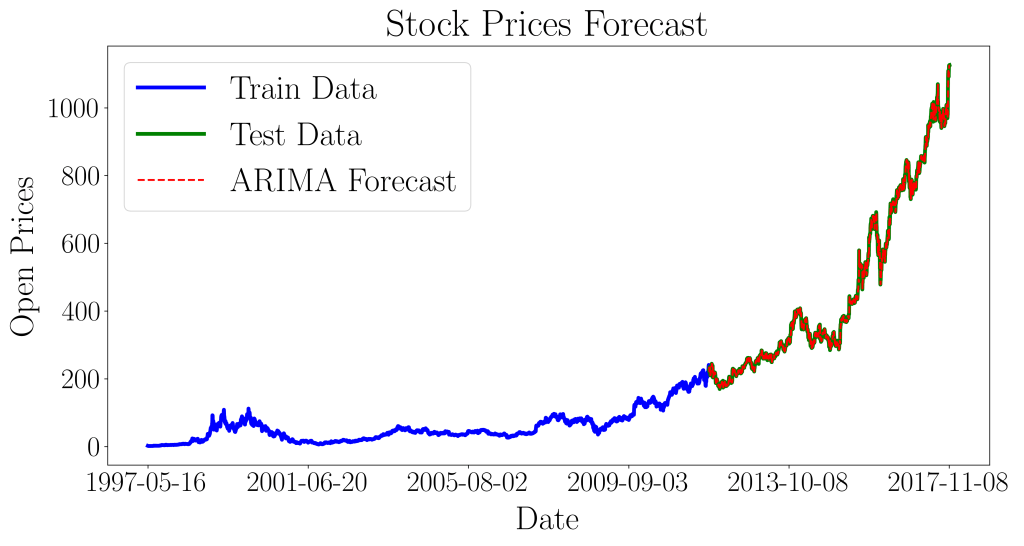
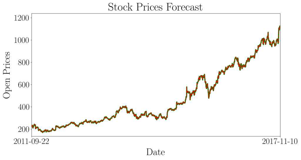
The forecast prices are very close to the actual prices, attaining a normalized mean squared error of 0.00069. Overall, our ARIMA model did pretty well in forecasting the stock prices for Amazon!

We hope that this real life application managed to pique your interest in applied statistics and statistical modeling. There are many more applications of such predictive methods and we can’t wait to share it with you in our future articles!