
Data science skills need not remain restricted to projects at work. Data can be found all around us, and when used effectively, data can help us answer questions, make decisions, and solve problems in our daily lives. One situation that may benefit from data-driven decision-making is choosing a neighborhood when relocating. In this post, we will leverage data about the neighborhoods of Singapore, ranked #1 in Asia and #25 in the world in Mercer’s 2019 Quality of Living Index. We will use data scraped from Wikipedia to get an idea of what neighborhoods can be found in Singapore, and we will use location data from Foursquare to cluster neighborhoods according to what types of venues can be found within. We will also visualize and interpret our results. Ultimately, our objective is showing how to use data science, along with a little critical thinking and creativity, to construction solutions to everyday problems.
We’ll start by importing some key Python libraries.
import pandas as pd
import numpy as np

from bs4 import BeautifulSoup # Library for web scrapping
import requests # Library to handle requests

from pandas.io.json import json_normalize # Use for tranforming json file into a pandas dataframe library

# Use for cluster analysis
from sklearn.cluster import KMeans
from sklearn import metrics
from scipy.spatial.distance import cdist
import matplotlib.pyplot as plt

# Libraries for displaying images
from IPython.display import Image
from IPython.core.display import HTML

# !conda install -c conda-forge folium=0.5.0 --yes
import folium # Helpful for making maps

# Tools for making plots
import matplotlib as mpl
import matplotlib.pyplot as plt
import matplotlib.cm as cm
import matplotlib.colors as colors
import seaborn as sns
Gathering Data through Web Scraping
Let’s gather some information about the neighborhoods of Singapore from public sources. We’ll scrape this from a Wikipedia page about Singapore neighborhoods using the BeautifulSoup package. The Wikipedia page includes two tables of neighborhoods that we must import and then append together in order to get our final dataset. Ultimately, we see that there are 26 main neighborhoods in Singapore.
First, we read in our two tables from Wikipedia.
# Getting data from wikipedia
wikipedia_link='https://en.wikipedia.org/wiki/New_towns_of_Singapore'
raw_wikipedia_page= requests.get(wikipedia_link).text

# Using BeautifulSoup to parse the HTML/XML codes
soup = BeautifulSoup(raw_wikipedia_page,'xml')
soup.prettify()

# Extracting the raw table inside that webpage
table = soup.find_all('table', {'class':'wikitable sortable'})

# Read in the first table and convert to a dataframe
df_General_InfoA = pd.read_html(str(table[0]), index_col=None, header=0)[0]
df_General_InfoA.head()

# Read in the second table and convert to a dataframe
df_General_InfoB = pd.read_html(str(table[1]), index_col=None, header=0)[0]
df_General_InfoB.head()
| Name (English/Malay) | Chinese | Pinyin | Tamil | Total area (km2) | Residential area (km2) | Dwelling units | Projected ultimate | Population | |
|---|---|---|---|---|---|---|---|---|---|
| 0 | Ang Mo Kio | 宏茂桥 | hóngmàoqiáo | ஆங் மோ கியோ | 6.38 | 2.83 | 49169 | 58000 | 149800 |
| 1 | Bedok | 勿洛 | wùluò | பிடோ | 9.37 | 4.18 | 60115 | 79000 | 204300 |
| 2 | Bishan | 碧山 | bìshān | பீஷான் | 6.90 | 1.72 | 19664 | 34000 | 65700 |
| … | … | … | … | … | … | … | … | … | … |
| 22 | Yishun | 义顺 | yìshùn | யீஷூன் | 7.78 | 3.98 | 56698 | 84000 | 186600 |
| Name (English/Malay) | Chinese | Pinyin | Tamil | Dwelling units | Population | |
|---|---|---|---|---|---|---|
| 0 | Bukit Timah | 武吉知马 | – | புக்கித் திமா | 2423 | 88000 |
| 1 | Marine Parade | 马林百列 | – | மரின் பரேட் | 6537 | 34300 |
| 2 | Central Area | 新加坡中區 | – | சிங்கப்பூர் மாவட்டம் | 9459 | 23300 |
Second, we combine our two tables from Wikipedia into one, resulting in a single pandas dataframe for us to work with.
# Reformat second table so it can be appended to the first
df_General_InfoB.insert(4, "Total area (km2)", np.nan)
df_General_InfoB.insert(5, "Residential area (km2)", np.nan)
df_General_InfoB.insert(7, "Projected ultimate", np.nan)
df_General_InfoB

# Combine the two tables into one
df_General_Info = df_General_InfoA.append(df_General_InfoB, ignore_index = True, sort = False)
df_General_Info
| Name (English/Malay) | Chinese | Pinyin | Tamil | Total area (km2) | Residential area (km2) | Dwelling units | Projected ultimate | Population | |
|---|---|---|---|---|---|---|---|---|---|
| 0 | Ang Mo Kio | 宏茂桥 | hóngmàoqiáo | ஆங் மோ கியோ | 6.38 | 2.83 | 49169 | 58000 | 149800 |
| 1 | Bedok | 勿洛 | wùluò | பிடோ | 9.37 | 4.18 | 60115 | 79000 | 204300 |
| … | … | … | … | … | … | … | … | … | … |
| 25 | Central Area | 新加坡中區 | – | சிங்கப்பூர் மாவட்டம் | NaN | NaN | 9459 | NaN | 23300 |
Gathering Data through APIs
Foursquare is a location technology platform that provides data about places (also called venues). For each venue, Foursquare can provide coordinates (i.e., latitude and longitude of the venue) as well as details, such as the type of venue (restaurant, store, gym, park, etc.), number of check-ins at the venue, and photos of the venue. By creating a Foursquare free developer account, we can use the Foursquare API to obtain basic information about venues in each neighborhood of Singapore.
An API, or application programming interface, allows users to request data from a software, web service, etc. What’s the difference between gathering data via web scraping vs. gathering data via an API? Previously, we could use web scraping to pull data from the Wikipedia page about Singapore neighborhoods because the data we wanted was displayed on the webpage. Now, we want to pull data from within Foursquare, so we need to use an API to send our data request.
First, you’ll need to define your Foursquare credentials. (Once you’ve created your free developer account, you can find these credentials in your account details.)
# Write your credentials here
CLIENT_ID = 'XXX' # your Foursquare ID
CLIENT_SECRET = 'XXX' # your Foursquare Secret

# Specify Foursquare version
VERSION = '20200816' # in YYYMMDD format
Second, we need to capture and import the latitude and longitude coordinates for the center of each neighborhood in Singapore. Soon, we’ll be using the Foursquare API to search for venues within a 500 meter radius of each neighborhood center, and we must provide the latitude and longitude coordinates of those neighborhood centers in our requests to Foursquare API. Google Maps provides a convenient way to pull latitude and longitude coordinates, and we then import these as a pandas dataframe.
# Read in dataset
df_Location = pd.read_csv("Data_Locations.csv")
df_Location.head()
| Town | Latitude | Longitude | |
|---|---|---|---|
| 0 | Ang Mo Kio | 1.369115 | 103.845436 |
| 1 | Bedok | 1.323604 | 103.927338 |
| … | … | … | … |
Third, we’ll write a function to extract a list of the venues in each neighborhood using Foursquare API. We start with our Location dataset, which includes the latitude and longitude coordinates of each neighborhood’s center, then we connect to the Foursquare API to find all venues within a 500 meter radius of each neighborhood center. This returns a json file containing the venues in each neighborhood, including their coordinates and categories (Park, Café, Supermarket, etc.), which we then convert into a pandas dataframe.
# Write function
def getNearbyVenues(names, latitudes, longitudes, radius=500, limit=8000):

    venues_list=[]
    for name, lat, lng in zip(names, latitudes, longitudes):
        print(name)

        # create the API request URL
        url = 'https://api.foursquare.com/v2/venues/explore?&client_id={}&client_secret={}&v={}&ll={},{}&radius={}&limit={}'.format(
            CLIENT_ID,
            CLIENT_SECRET,
            VERSION,
            lat,
            lng,
            radius,
            limit)

        # make the GET request
        results = requests.get(url).json()['response']['groups'][0]['items']

        # return only relevant information for each nearby venue
        venues_list.append([(
            name,
            lat,
            lng,
            v['venue']['name'],
            v['venue']['location']['lat'],
            v['venue']['location']['lng'],
            v['venue']['categories'][0]['name']) for v in results])

    nearby_venues = pd.DataFrame([item for venue_list in venues_list for item in venue_list])
    nearby_venues.columns = ['Neighborhood',
                  'Neighborhood Latitude',
                  'Neighborhood Longitude',
                  'Venue',
                  'Venue Latitude',
                  'Venue Longitude',
                  'Venue Category']

    return(nearby_venues)

# Use function
df_Nearby_Venues_Raw = getNearbyVenues(names=df_Location['Town'],
                                   latitudes=df_Location['Latitude'],
                                  longitudes=df_Location['Longitude']
                                  )
| Neighborhood | Neighborhood Latitude | Neighborhood Longitude | Venue | Venue Latitude | Venue Longitude | Venue Category | |
|---|---|---|---|---|---|---|---|
| 0 | Ang Mo Kio | 1.369115 | 103.845436 | Kam Jia Zhuang Restaurant | 1.368167 | 103.844118 | Asian Restaurant |
| 1 | Ang Mo Kio | 1.369115 | 103.845436 | Old Chang Kee | 1.369094 | 103.848389 | Snack Place |
| … | … | … | … | … | … | … | … |
Data Restructuring
Before we use the data we’ve gathered from Foursquare to run a cluster analysis, we’ll explore and restructure the data a bit. This step is critical because although data is easy to find, it is rarely in a format ideal for analyzing. Transforming raw data into suitable input for a model often requires some resourcefulness. In the current case, there are two aspects of the dataset that we must alter before we can use it as input for K-Means Clustering:
- Change string data to numeric data using one-hot encoding, because K-Means Clustering requires input data to be numeric
- Group by neighborhood such that each row reflects one neighborhood rather than one venue, because K-Means Clustering sorts rows into clusters, and we want to cluster neighborhoods, not venues
Exploring the Data
# Examine the shape of the dataset (how many rows and columns)
df_Nearby_Venues_Raw.shape

# Determine the number of unique venue types in the dataset (restaurants, bakeries, yoga studios, etc.)
print('There are {} uniques categories.'.format(len(df_Nearby_Venues_Raw['Venue Category'].unique())))

# See how many venues are found in each neighborhood
df_Nearby_Venues_Raw.groupby('Neighborhood').count()
One-Hot Encoding
One-hot encoding allows us to restructure the data such that instead of having a single “Venue Category” feature (column) specifying the category of each venue (row), we now have one feature (column) per category of venue (“Wine Bar,” “Yoga Studio,” etc.). For each venue (row), each of these new features (columns) is coded dichotomously: 0 means the venue does not fall into the given category; 1 means the venue does fall into the given category.
# One-hot encoding
df_Nearby_Venues_OneHot = pd.get_dummies(df_Nearby_Venues_Raw[['Venue Category']], prefix="", prefix_sep="")

# Add neighborhood column back to dataframe
df_Nearby_Venues_OneHot['Neighborhood'] = df_Nearby_Venues_Raw['Neighborhood']

# Move neighborhood column to the first column
fixed_columns = [df_Nearby_Venues_OneHot.columns[-1]] + list(df_Nearby_Venues_OneHot.columns[:-1])
df_Nearby_Venues_OneHot = df_Nearby_Venues_OneHot[fixed_columns]

# Checking
df_Nearby_Venues_OneHot.head()
| Neighborhood | Accessories Store | Art Gallery | Asian Restaurant | … | Waterfront | Wings Joint | Yoga Studio | |
|---|---|---|---|---|---|---|---|---|
| 0 | Ang Mo Kio | 0 | 0 | 1 | … | 0 | 0 | 0 |
| 1 | Ang Mo Kio | 0 | 0 | 0 | … | 0 | 0 | 0 |
| … | … | … | … | … | … | … | … | … |
Grouping by Neighborhood
Next, we group our dataset by neighborhood. In our one-hot encoded dataset, each row corresponds to one venue, but we want each row to correspond to one neighborhood. Grouping by neighborhood and calculating each feature as “sum of the frequency of occurrence of each category” will show each neighborhood along with how many venues it has in each category.
df_Nearby_Venues_Grouped = df_Nearby_Venues_OneHot.groupby('Neighborhood').sum().reset_index()
| Neighborhood | Accessories Store | Art Gallery | Asian Restaurant | … | Waterfront | Wings Joint | Yoga Studio | |
|---|---|---|---|---|---|---|---|---|
| 0 | Ang Mo Kio | 0 | 0 | 2 | … | 0 | 0 | 0 |
| 1 | Bedok | 0 | 0 | 2 | … | 0 | 1 | 0 |
| … | … | … | … | … | … | … | … | … |
| 25 | Yishun | 0 | 0 | 0 | … | 0 | 0 | 0 |
Cluster Analysis
We now leverage K-Means Clustering, which uses our numeric features (i.e., how many venues in each category) to group similar neighborhoods together. K-Means Clustering sorts observations into a specified number of groups (k) using randomly initialized “center points,” which are iteratively re-centered until clusters stabilize around them. The algorithm attempts to minimize the variance within clusters while maximizing the distance between clusters. In our current analysis, the objective of the K-Means Clustering is to cluster neighborhoods that are similar to each other with respect to their most common venue types while ensuring the clusters of neighborhoods differ meaningfully from each other. For example, neighborhoods that contain many coffee shops may be sorted into one cluster, and this cluster will differ from other clusters wherein neighborhoods have fewer coffee shops.
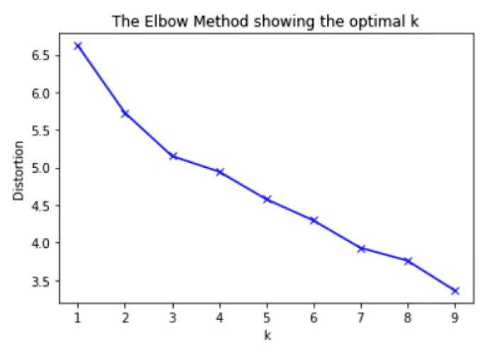
K-Means Clustering requires the user to specify how many clusters the model should find, so we first generate an “elbow graph” to show the optimal number clusters to use. There’s not a very clear “elbow” in our plot, so we select 4 clusters (the middle point).
# Data for clustering
Sing_Cluster_Data = df_Nearby_Venues_Grouped.drop('Neighborhood', 1)
Sing_Cluster_Data.head()

# K-means determine k
distortions = []
K = range(1,10)
for k in K:
    ChooseKModel = KMeans(n_clusters=k).fit(Sing_Cluster_Data)
    ChooseKModel.fit(Sing_Cluster_Data)
    distortions.append(sum(np.min(cdist(Sing_Cluster_Data, ChooseKModel.cluster_centers_, 'euclidean'), axis=1)) / Sing_Cluster_Data.shape[0])

# Plot the elbow
plt.plot(K, distortions, 'bx-')
plt.xlabel('k')
plt.ylabel('Distortion')
plt.title('The Elbow Method showing the optimal k')
plt.show()
Next, the algorithm sorts our 26 neighborhoods into 4 clusters.
# Set number of clusters
kclusters = 4

# Run k-means clustering
ClusterModel = KMeans(n_clusters=kclusters, random_state=0).fit(Sing_Cluster_Data)

# Check cluster labels generated for each row in the dataframe
ClusterModel.labels_[0:27]
| Cluster | Neighborhoods |
|---|---|
| 0 | Bedok, Jurong East, Jurong West, Tampines, Woodlands |
| 1 | Bukit Merah, Bukit Panjang, Bukit Timah, Kallang/Whampoa, Marine Parade, Punggol, Queenstown, Sembawang, Sengkang, Serangoon |
| 2 | Ang Mo Kio, Bishan, Bukit Batok, Choa Chu Kang, Clementi, Geylang, Hougang, Pasir Ris, Toa Payoh, Yishun |
| 3 | Central |
Finally, we’ll create a new dataset that includes the elements listed below; this dataset shows what types of venues are most common in each neighborhood and will help us interpret our results later.
- Neighborhood names
- Coordinates of each neighborhood (latitude / longitude)
- Cluster label for each neighborhood
- Top 10 common venues for each neighborhood
# Create function to sort venues in descending order
def return_most_common_venues(row, num_top_venues):
    row_categories = row.iloc[1:]
    row_categories_sorted = row_categories.sort_values(ascending=False)

    return row_categories_sorted.index.values[0:num_top_venues]

num_top_venues = 10

indicators = ['st', 'nd', 'rd']

# create columns according to number of top venues
columns = ['Neighborhood']
for ind in np.arange(num_top_venues):
    try:
        columns.append('{}{} Most Common Venue'.format(ind+1, indicators[ind]))
    except:
        columns.append('{}th Most Common Venue'.format(ind+1))

# create a new dataframe
df_Nearby_Venues_Sorted = pd.DataFrame(columns=columns)
df_Nearby_Venues_Sorted['Neighborhood'] = df_Nearby_Venues_Grouped['Neighborhood']

for ind in np.arange(df_Nearby_Venues_Grouped.shape[0]):
    df_Nearby_Venues_Sorted.iloc[ind, 1:] = return_most_common_venues(df_Nearby_Venues_Grouped.iloc[ind, :], num_top_venues)

# Add clustering labels to "Most Common Venue Types, by Neighborhood" dataset
df_Nearby_Venues_Sorted.insert(0, 'Cluster Labels', ClusterModel.labels_)

# Prep Location dataset
df_Neighborhoods_Merged = df_Location

# Merge venue data with latitude/longitude for each neighborhood
df_Neighborhoods_Merged = df_Neighborhoods_Merged.join(df_Nearby_Venues_Sorted.set_index('Neighborhood'), on='Town')
| Neighborhood | Latitude | Longitude | Cluster Labels | 1st Most Common Venue | 2nd Most Common Venue | … | 9th Most Common Venue | 10th Most Common Venue | |
|---|---|---|---|---|---|---|---|---|---|
| 0 | Ang Mo Kio | 1.369115 | 103.845436 | 2 | Food Court | Coffee Shop | … | Sandwich Place | Asian Restaurant |
| 1 | Bedok | 1.323604 | 103.927338 | 0 | Café | Chinese Restaurant | … | Japanese Restaurant | Malay Restaurant |
| … | … | … | … | … | … | … | … | … | … |
| 25 | Yishun | 1.430400 | 103.835400 | 2 | Food Court | Italian Restaurant | … | Supermarket | Restaurant |
Visualizing and Interpreting Results
Now, we now need to make sense of our results. First, we’ll create a map of Singapore with neighborhoods color-coded by cluster according to the results of our K-Means Cluster analysis. Second, we’ll create some basic graphs and plots based on the neighborhood information we scraped from Wikipedia. Third, we’ll examine what types of venues are common across the neighborhoods assigned to each cluster to interpret our four clusters.
Mapping Neighborhoods
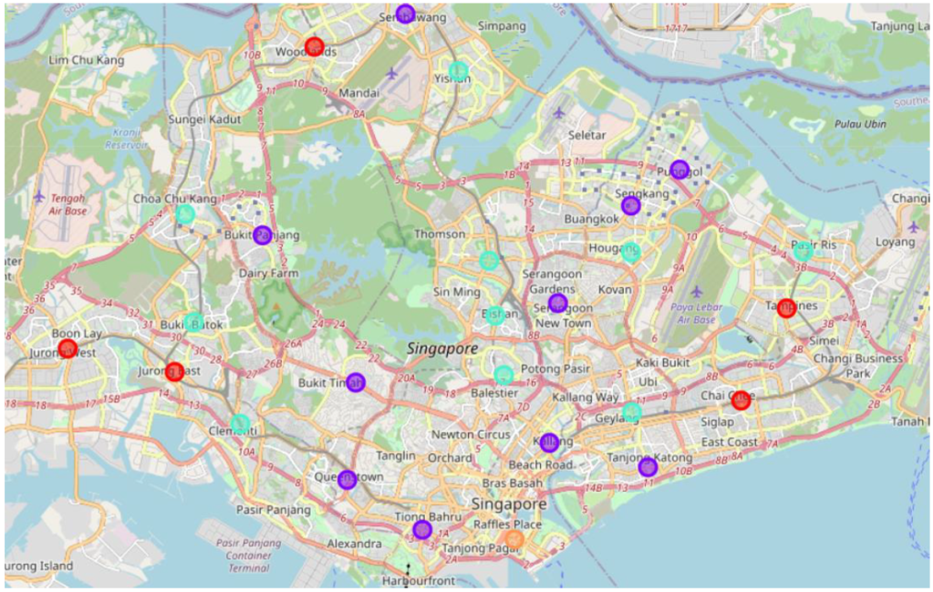
Maps allow us to consume a large amount of information at a glance, making them a useful type of data visualization. Using the Folium Python package for map-making, we visualize the neighborhoods of Singapore on a map. Cluster 1 (in purple) and Cluster 2 (in teal) each contain 10 neighborhoods, Cluster 0 (in red) contains 5 neighborhoods, and Cluster 3 (in orange) contains only one neighborhood (Central).
# Create map of Singapore using lat and long coordinates
latitude = 1.3521
longitude = 103.8198
Map_Clusters = folium.Map(location=[latitude, longitude], zoom_start=12)

# Set color scheme for the clusters
x = np.arange(kclusters)
ys = [i + x + (i*x)**2 for i in range(kclusters)]
colors_array = cm.rainbow(np.linspace(0, 1.2, len(ys)))
rainbow = [colors.rgb2hex(i) for i in colors_array]

# Add markers to the map
markers_colors = []
for lat, lon, poi, cluster in zip(df_Neighborhoods_Merged['Latitude'], df_Neighborhoods_Merged['Longitude'], df_Neighborhoods_Merged['Town'], df_Neighborhoods_Merged['Cluster Labels']):
    label = folium.Popup(str(poi) + ' Cluster ' + str(cluster), parse_html=True)
    folium.CircleMarker(
        [lat, lon],
        radius=8,
        popup=label,
        color=rainbow[cluster-1],
        fill=True,
        fill_color=rainbow[cluster-1],
        fill_opacity=0.5).add_to(Map_Clusters)
Graphs and Plots
Graphs and plots provide another means of data visualization. In this case, we’ll use our general data about the neighborhoods of Singapore that we scraped from Wikipedia. We’ll use a column graph and a scatterplot to examine population density in Singapore’s neighborhoods. Let’s start with the scatterplot.
# Scatterplot: Total Area (km2) x Population
sns.relplot(x='Total area (km2)', y='Population', color="red", data=df_General_Info)
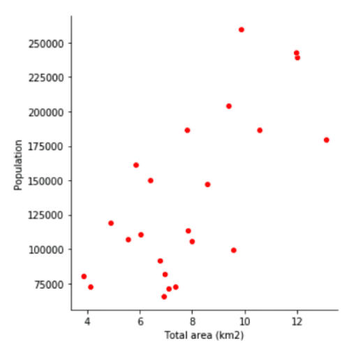
Examining our scatterplot, we see a clear relationship between population and total area (in square kilometers) across neighborhoods of Singapore. In other words, neighborhoods that are larger in area also tend to be larger in terms of population.
Next, we’ll look at the population density for each neighborhood to identify the most and least densely populated neighborhoods.
# Column Chart: Population Density (Population / Total Area [km2])

# Create population density dataset
Pop_Density = df_General_Info['Population'] / df_General_Info['Total area (km2)']
df_Pop_Density = pd.DataFrame(Pop_Density)
df_Town = df_General_Info[["Name (English/Malay)"]]
df_Pop_Density.insert(0, "Neighborhood", df_Town)
df_Pop_Density.columns = ["Neighborhood","Population Density"]

# Graph
sns.barplot(df_Pop_Density['Neighborhood'],df_Pop_Density['Population Density'], color='red', order=df_Pop_Density.sort_values('Population Density')['Neighborhood'])
plt.xticks(rotation=-45, ha='left')
plt.ylabel('Population Density (Population / Total Area)')
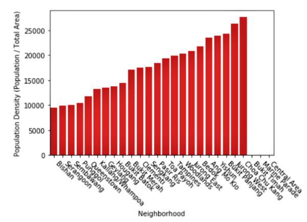
Inspecting our column graph, we see that Bishan is the least densely populated neighborhood in Singapore with just under 10,000 people per square kilometer. In contrast, Choa Chu Kang is the most densely populated neighborhood in Singapore with over 25,000 people per square kilometer. For comparison, the population density of Manhattan, New York City is 25,846 people per square kilometer (according to Wikipedia).
Interpreting Results
To better understand the results of the cluster analysis and determine what characterizes each cluster of neighborhoods, we’ll examine trends in the top 10 most common venues types for neighborhoods within each cluster
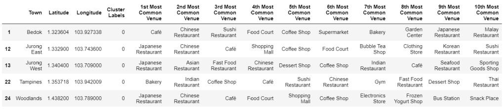
Cluster 0: Save Room for Dessert
Cluster 0 contains 5 neighborhoods: Bedok, Jurong East, Jurong West, Tampines, and Woodlands. In 3 out of the 5 neighborhoods, the 1st most common venue type is “Japanese Restaurant.” All 5 neighborhoods have some variety of restaurant as the 2nd most common venue type (“Chinese Restaurant,” “Asian Restaurant,” or “Indian Restaurant”), and all 5 neighborhoods have “Café” included at some point in their top 10 most common venue types. In addition, each of the 5 neighborhoods includes some form of sweets shop in its top 10 most common venue types: “Bakery,” “Bubble Tea Shop,” “Dessert Shop,” “Frozen Yogurt Shop.” Overall, food-related venues—especially cafés and shops selling sweets—are featured prominently in neighborhoods of this cluster.
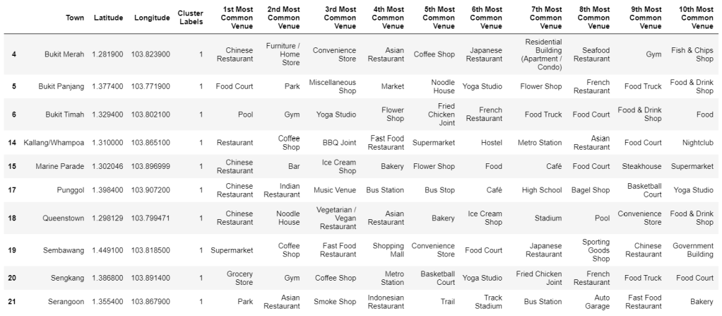
Cluster 1: Lively and Fit
Cluster 1 contains 10 neighborhoods: Bukit Merah, Bukit Panjang, Bukit Timah, Kallang/Whampoa, Marine Parade, Punggol, Queenstown, Sembawang, Sengkang, and Serangoon. In 4 out of the 10 neighborhoods, the 1st most common venue type is “Chinese Restaurant.” Another 2 neighborhoods have a 1st most common venue type of “Food Court” or “Restaurant,” and an additional 2 neighborhoods have a 1st most common venue type of “Grocery Story” or “Supermarket.” The final two neighborhoods have a 1st most common venue type of “Park” or “Pool.” Fitness emerges as a key theme among the most common venues of Cluster 1, with entries such as “Gym,” “Yoga Studio,” “Basketball Court,” “Track Stadium,” “Trail,” and “Sporting Goods Shop.” Cluster 1 also suggests a trendy vibe, with venues such as “Nightclub,” “Bar,” and “Music Venue.”
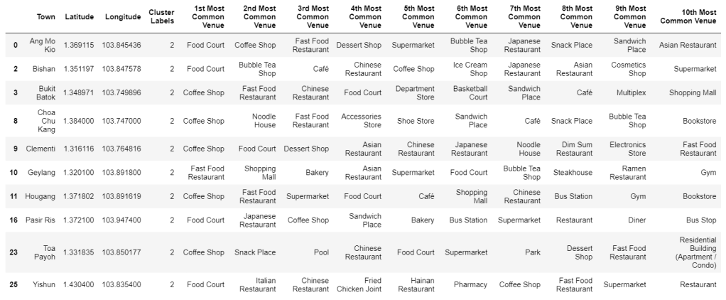
Cluster 2: Shop and Eat Local
Cluster 2 also contains 10 neighborhoods: Ang Mo Kio, Bishan, Bukit Batok, Choa Chu Kang, Clementi, Geylang, Hougang, Pasir Ris, Toa Payoh, and Yishun. In 9 out of the 10 neighborhoods, the 1st most common venue type is “Food Court” or “Coffee Shop.” (The final neighborhood has “Fast Food Restaurant” as its most common venue type.) In fact, “Coffee Shop” and “Food Court” each appear in the top 10 most common venue types lists in 9 out of the 10 neighborhoods. Looking to the rest of the common venue types across neighborhoods of Cluster 2, shopping and leisure seem prominent, with “Cosmetics Shop,” “Department Store,” “Shopping Mall,” “Bookstore,” Shoe Store,” “Electronics Store,” “Accessories Store,” and “Multiplex” all appearing.
Cluster 3: Downtown
Cluster 3 contains only one neighborhood: Central. Its most common venue type is “Japanese Restaurant,” followed by “Coffee Shop.” The Central neighborhood’s top 10 most common venue types list does not include casual dining options such a “Food Court” or “Fast Food Restaurant.” Instead, the Central neighborhood has a more upscale feel, with “Hotel” and “Bar” appearing as common venues.

Conclusion
In this post, we’ve demonstrated several techniques for applying data science to everyday life:
- Scraping data from Wikipedia
- Using Foursquare API to gather location data about venues within neighborhoods
- Clustering the neighborhoods according to what types of venues are found within
- Visualizing and and interpreting results
We hope you will find this content illuminating as you think of creative ways to leverage data science in your day-to-day life!
