
Deep learning is part of a broader spectrum of machine learning methods known as artificial neural networks. It can be trained on both supervised and unsupervised data, and has proven to be an effective modeling tool in both linear and non-linear contexts. A widely used deep learning library is Keras — a high-level neural networks API, written in Python, capable of running on top of TensorFlow, CNTK, or Theano. Today, we introduce concepts of deep learning with a demonstration, in the hope that by the end of the article, the reader will have a better understanding of how deep learning algorithms work, and how to implement your very own neural network!
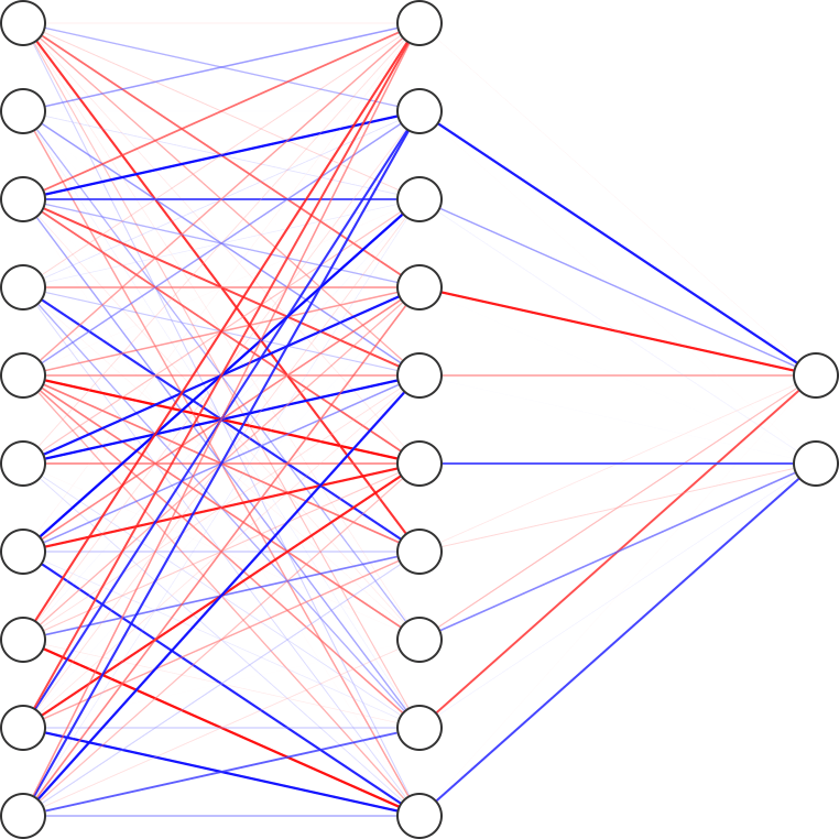
We show a sample neural network with three layers: input layer (10 nodes), hidden layer (10 nodes), and output layer (2 nodes). All layers between the input and output layers are called hidden layers. This visualization allows us to have a better understanding about the interaction between the different nodes, and a visualization of the weights associated with each edge. The boldness of the line represents the magnitude of the weights, and color represents the sign of the weights (red is negative and blue is positive).
To make things more challenging, we will be using a slightly imbalanced data set with 80% outcomes of 0 and 20% outcomes of 1. This data set can be downloaded here, and its poor performance using random forest can be seen in a previous article. Imbalanced data sets have often been thought to be a curse for machine learning algorithms. The ability for the machine learning model to pick up the minority outcomes, in areas such as fraud detection, is critical but challenging. The performance of the deep learning neural network and its ability to tackle an imbalanced data set will be revealed at the end of this exercise! The deep learning demonstration using Keras is as follows.
- Data Loading: Load the csv file using Pandas and discuss the intricacies of Keras inputs.
- Data Manipulation: Split the data into 70% training set and 30% validation set.
- Model Training: Build and train the neural networks with the training data. The various parameters for tuning the model will be introduced and explained.
- Model Validation: Test the model’s predictive power by applying it to the validation set.
Data Loading
The data is read using pandas.read_csv. X here refers to the predictors and y refers to outcomes (0 or 1).
def read_data():

    # Read csv file
    df = pd.read_csv('clean_data.csv')

    # Transform data into predictors 'X' and outcome 'y'
    X = df.drop('y', axis=1).values
    y = df['y'].values

    return df, np.array(X), np.array(y)
The csv file is at this point converted to a pandas data frame, which is unfortunately incompatible with Keras function calls. Keras expects its inputs to be a NumPy array and this conversion can be achieved by calling np.array with the data frame as the input. These will be used as inputs for the Keras functions for building the model.
Data Manipulation
In order to validate our model, we split the data set into 70% training set and 30% validation set. We use train_test_split from scikit-learn to achieve this. A constant seed number called SEED is given to the function for reproducible results.
def split_data(X, y):
    from sklearn.model_selection import train_test_split

    # Split dataset into 70% train, 30% test
    X_train, X_test, y_train, y_test = train_test_split(X, y,
                                                   test_size=0.3,
                                                   stratify=y,
                                                   random_state=SEED)
    return X_train, X_test, y_train, y_test
Model Training
This section will be divided into the following subsections, to facilitate the explanation of how the deep learning algorithm works, while showing the implementation using Keras.
- Defining Keras Model: Defines the type of neural network structure.
- Building Network Layers: Adding layers of neural network, and initializing the appropriate number of input and output nodes.
- Compiling Keras Model: Compiles the Keras model with numerical libraries such as Theano or TensorFlow. Defining input parameters such as type of optimizer, loss function, and performance metric to be used.
- Checkpointing in Keras: Saving the best model parameters found during the training process. This allows the user to load the stored parameters for later use.
- Fit Keras model: Training the model with the training set, and defining training parameters such as
epochsandbatch_size.
Defining Keras Model
from keras.models import Sequential

# Initialize sequential model
model = Sequential()
There are two main types of models in Keras: Sequential and Model (functional API). The Keras Sequential model is a linear stack of neural network layers while the Keras Model functional API defines complex models, such as multi-input/-output models, directed acyclic graphs, or models with shared layers. In most cases, a Sequential model would be the first thing to try, and if deemed unsatisfactory, the user can resort to more complex models.
Building Network Layers
Note that having a linear stack of neural networks does not imply that it cannot model non-linear interactions. The non-linear interactions do not depend on the structure of the layers, but rather the interaction between the nodes defined by the activation function. The activation function decides whether a node should be activated or not by calculating the weighted sum and further adding bias with it. The purpose of the activation function is to introduce non-linearity into the output of a node.
The code below implements the 3 layers of neural network and we will explain the choice of the input parameters in detail.
from keras.layers import Dense

# Number of predictors
n_cols = X_train.shape[1]

# Input layer
model.add(Dense(100, activation='relu', input_shape = (n_cols,)))
# Hidden layer
model.add(Dense(n_cols, activation='relu'))
# Output layer
model.add(Dense(1, activation='sigmoid'))
All layers are defined using Keras’s Dense, to indicate a layer of dense neural network. It is so called densely connected because each node receives input from all the nodes in the previous layer. The first (input) layer has 100 nodes, and the number of predictors is given to input_shape. This input_shape needs to be defined only for the first layer. Here, the second layer (also known as the first hidden layer) has the same number of nodes as input_shape. And finally the output only has one node, giving a result in terms of probabilities, with regards to the classification type of each data point.
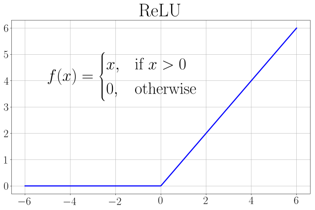
After understanding the input parameters regarding the number of nodes, we move on to discuss the choice of activation functions. ReLU (rectified linear unit) is chosen for the first two layers because it is computationally more efficient (compared to sigmoid or tanh), and much better gradient propagation (resulting in fewer vanishing gradient problems compared to using sigmoid).
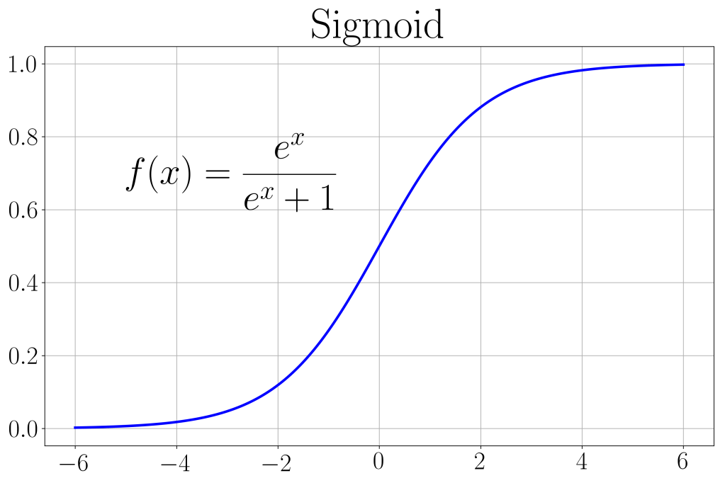
The output activation function is chosen to be a sigmoid. It is an S-shaped curve ranging between [0, 1] as shown. We use this function so that predictions can range between [0, 1], which can then be easily converted to the binary classification using the threshold of 0.5.
Compiling Keras Model
The following code defines three input parameters: optimizer, loss, and metrics. The choice of optimizer refers to the algorithm chosen for the deep learning model. A good optimizer is one which is cost effective, yet accurate. A favored choice is the “adam” optimizer, adapted from the classical stochastic gradient descent method for the purpose of updating network weights iteratively based on training data. While classical stochastic gradient descent maintains one single learning rate for all weight updates throughout the training process, “adam” has a separate learning rate for each network weight and updates it iteratively throughout the training process. It is popular among deep learning algorithms due to its good performance and high computational efficiency.
# Compile
model.compile(optimizer='adam',
              loss='binary_crossentropy',
              metrics=['accuracy'])
The binary cross entropy loss function is the loss function to be used for binary classification problems (usually labelled 0 and 1). Cross entropy calculates an index which summarizes the difference between the actual and predicted probability distributions for predicting class 1. This loss function produces a value that ranges [0, 1] and the lower the loss, the more accurate the model. As for the performance metrics, we chose classification accuracy as the metric to be reported since it’s a classification problem.
Checkpointing in Keras
Checkpointing allows Keras to store the best parameters (network weights) during the training process, in the event where the model starts to perform poorly as the training progresses. One may wonder, in what scenario will more training result in a model with poorer predictive power? The answer: an over-fitted model. More training can sometimes lead to over-fitting of the training data set, resulting in a model with poor validation scores. In the code below, we inform Keras to store the best parameters in the file best_model.h5 (a HDF5 data file) , with the monitoring performance metric set as the loss value for the validation set (val_loss). Since a smaller loss value, implies a more accurate model, we set mode=min implying that we would like to minimize the loss value for the validation set. By setting save_best_only=True, only the best model parameters, as defined by our choice of performance metrics, are saved in the HDF5 file.
from keras.callbacks import ModelCheckpoint

# This checkpoint object will store the model parameters in the file "best_model.h5"
checkpoint = ModelCheckpoint('best_model.h5', monitor='val_loss', mode='min', save_best_only=True)

# Store in a list to be used during training
 callbacks_list = [checkpoint]
The checkpoint object we created is then stored in a list called callbacks_list for later use during model fitting. If one wishes to load the saved model parameters, the function keras.models.load_model will do the job, and you can use the model as it is without fitting/training!
Fit Keras Model
# Fit model to the training set
history = model.fit(X_train, y_train, validation_data=(X_test, y_test), batch_size=10, epochs=10, callbacks=callbacks_list)
The callbacks_list created previously is placed as an input for model fitting. This allows for close monitoring of model training, and the best parameters are then stored in callbacks_list. The train set (X_train, y_train) and validation set (X_test, y_test) are also passed into model.fit as inputs, for training and validating the model. Two new input parameters, integral to the training process are given below.
- epochs: number of complete passes through the training dataset. One forward pass and one backward pass of all training data constitutes a complete pass.
- batch_size: number of training samples to work through one forward/backward pass before the model’s parameters (network weights) are updated.
As an example, if we have 100 training data points, and batch size of 10, then each epoch will take 10 iterations. Epochs and batch sizes are in fact hyperparameters for the stochastic gradient descent algorithm in “adam”. Understanding these parameters tells us a few things: the higher the batch size, the more memory intensive it is; the higher the epoch, the more computationally expensive it gets. Since “adam” is an iterative optimization algorithm, several passes through the data set will be necessary to obtain good results. Therefore, we set the epochs=10 and batch_size=10. Since our data set has 40,000 rows of data, the number of training data (70%) is 28,000. With a batch size of 10, each epoch requires 2800 iterations. *Note that if batch size is unspecified, the default in Keras is set at 32.
The training history of the deep learning algorithm can be plotted out with the “loss” or “accuracy” against the epoch iteration.
# Plot training loss history
plt.plot(history.history['loss'], 'b', label='Training Set (Loss)', linewidth=3)
plt.plot(history.history['val_loss'], 'r', label='Validation Set (Loss)', linewidth=3)

# Plot training accuracy history
plt.plot(history.history['accuracy'], 'b', label='Training Set (Accuracy)', linewidth=3)
plt.plot(history.history['val_accuracy'], 'r', label='Validation Set (Accuracy)', linewidth=3)
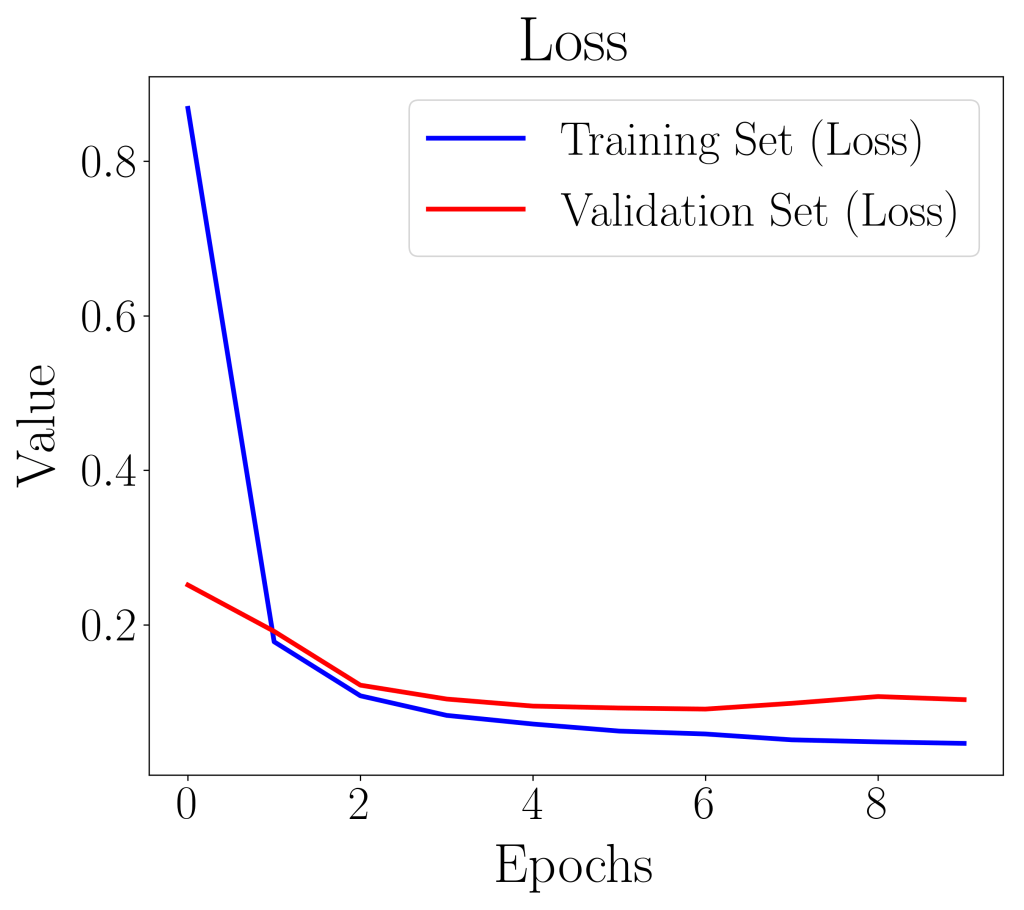
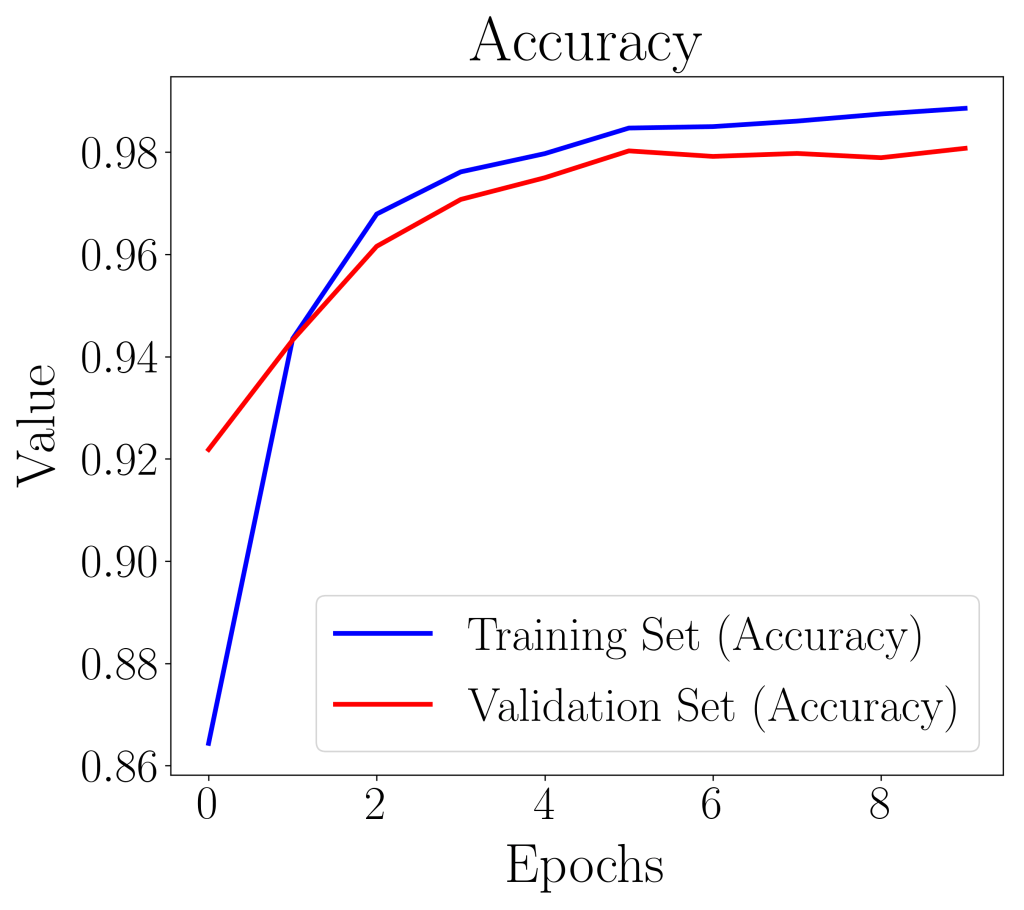
In the plot of loss value against epoch, if the validation loss curve starts increasing, it is a sign that the model has over-fitted. In our case, both the accuracy and loss plots suggest that our model is well-fitted and is ready to be evaluated with further metrics.
Model Validation
The AUC score reported below, shows that the train set and validation set have very similar AUC scores. This is an indication that the neural network model is well-fitted and is able to generalize to independent data sets.
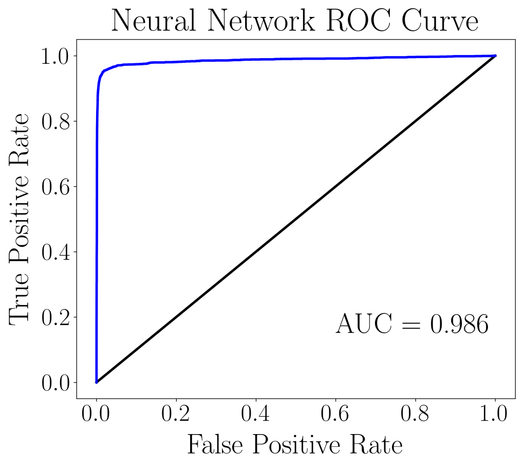
| Training Set | Validation Set | |
| AUC score | 0.995 | 0.986 |
Comparing this classification report with the random forest classifier and the balanced bootstrap random forest classifier from a previous article, we see that the deep learning neural network produces a model that performs better on imbalanced data sets. Interestingly, no tweaking is required on the part of the deep learning model, in order for the model to learn to predict the minority outcomes.
| Precision | Recall | Specificity | F1 | Geometric Mean | |
| 0 | 0.98 | 0.99 | 0.94 | 0.99 | 0.96 |
| 1 | 0.96 | 0.94 | 0.99 | 0.95 | 0.96 |
| Predicted | |||
| 0 | 1 | ||
| Actual | 0 | 9477 | 97 |
| 1 | 153 | 2273 |
The confusion matrix also suggests highly accurate predictions with very few mis-classifications (off-diagonals). None of the entries are extremely sparse, which usually is a sign of over-prediction of the majority outcome in imbalanced data sets. Overall, the deep learning neural network has performed very well and shows great promise in areas where imbalanced data sets are prevalent.
