
The curse of imbalanced data refers to machine learning models trained to predict outcomes which are majority, and neglecting the minority. This is a common problem in fraud detection, cancer classification, etc. In those examples, although the occurrence of the positive outcome is rare, it is highly crucial that the machine learning model is able to pick up those rare events. In a previous article, we saw that the random forest over-predicted the number of 0 outcomes, for a slightly imbalanced data set that has 80% outcomes with 0 and 20% with 1. This is not surprising, since the BaggingClassifier used in scikit-learn RandomForestClassifier, does not balance each sample of data. Without special treatment, the machine learning model is not able to train well on the minority outcomes. One way to fix the problem, is provide the RandomForestClassifier with a balanced bootstrap sample. In this way, even though the raw data is imbalanced, we balance the data by either under-sampling data with the majority outcome or over-sample data with the minority outcome, resulting in a balanced bootstrap sample for the machine learning model to train on.
This article will provide a demonstration, comparing between the
RandomForestClassifierfrom scikit-learn, with no special treatment for imbalanced data sets, andBalancedRandomForestClassifierfrom imbalanced-learn, which uses under-sampling to provide a balanced bootstrap sample for the classifier.
Numerical Demonstration
The numerical demonstration will be as follows:
- Data Manipulation: Split the data into 70% training set and 30% validation/hold-out set.
- Model Training: (1) RandomForestClassifier and (2) BalancedRandomForestClassifier, with the same set of hyperparameters.
- Model Validation: Test the models with the validation/hold-out data and compare their performance with suitably chosen accuracy metrics.
Data Manipulation
First, we read the data using pandas and store the predictors and outcome separately into X and y.
def read_data():

    # Read csv file
    df = pd.read_csv('clean_data.csv')

    # Transform data into predictors 'X' and outcome 'y'
    X = df.drop('y', axis=1).values
    y = df['y'].values
    return df, X, y
The function split_data then takes in the predictors X and outcome y and splits the data into train and test sets using scikit-learn’s train_test_split. We provide a constant random seed number so that the results simulated are reproducible.
def split_data(X, y):
    from sklearn.model_selection import train_test_split

    # Split dataset into 70% train, 30% test
    X_train, X_test, y_train, y_test = train_test_split(X, y,
                                                        test_size=0.3,
                                                        stratify=y,
                                                        random_state=SEED)
    return X_train, X_test, y_train, y_test
Model Training
Given the type_of_bootstrap, which can be “Balanced RF” or “RF”, the function train_model instantiates and trains the specified machine learning model with the training data set X_train, y_train. The same set of hyperparameters is provided to both machine learning models for a fair comparison.
def train_model(X_train, y_train, type_of_bootstrap):
    from sklearn.ensemble import RandomForestClassifier
    from imblearn.ensemble import BalancedRandomForestClassifier

    if type_of_bootstrap == 'Balanced RF':
        # Instantiate balanced random forest classifier 'rf'
        rf = BalancedRandomForestClassifier(n_estimators=50,
                                            random_state=SEED,
                                            n_jobs=-1)
    elif type_of_bootstrap == 'RF':
        # Instantiate random forest classifier 'rf'
        rf = RandomForestClassifier(n_estimators=50,
                                    random_state=SEED,
                                    n_jobs=-1)
    # Fit rf to the training set
    rf.fit(X_train, y_train)
    return rf
Model Validation
Lastly, we test each model with the validation/hold-out data set, and output the results for further post-process comparison between the two models.
def predict_validation(model, X_test, y_test, type_of_bootstrap):
    from sklearn.metrics import roc_curve

    # Predict test set labels
    y_pred = model.predict(X_test)

    # Retrieve probability for ROC curve
    y_pred_prob = model.predict_proba(X_test)[:,1]

    # Output probability results
    pd.DataFrame(y_pred_prob.T).to_csv('csv/%s-prob.csv'%type_of_bootstrap, index=False, header=False)

    fpr, tpr, thresholds = roc_curve(y_test, y_pred_prob)
    return fpr, tpr, y_pred, y_pred_prob
Comparison between RandomForestClassifier and BalancedRandomForestClassifier: What metrics to use?
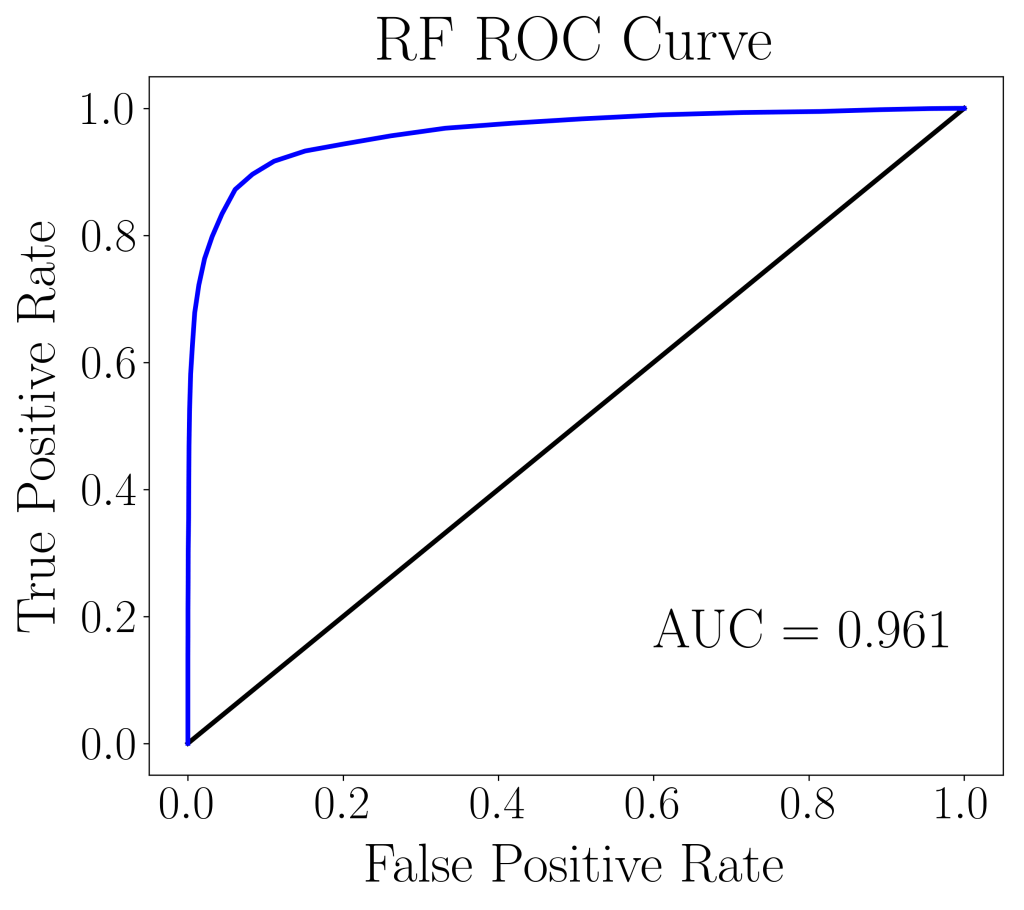
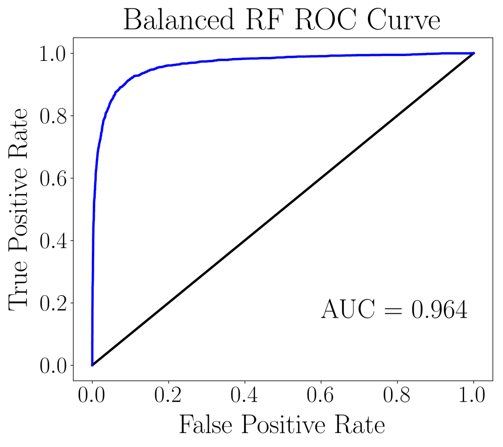
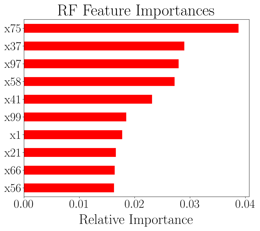
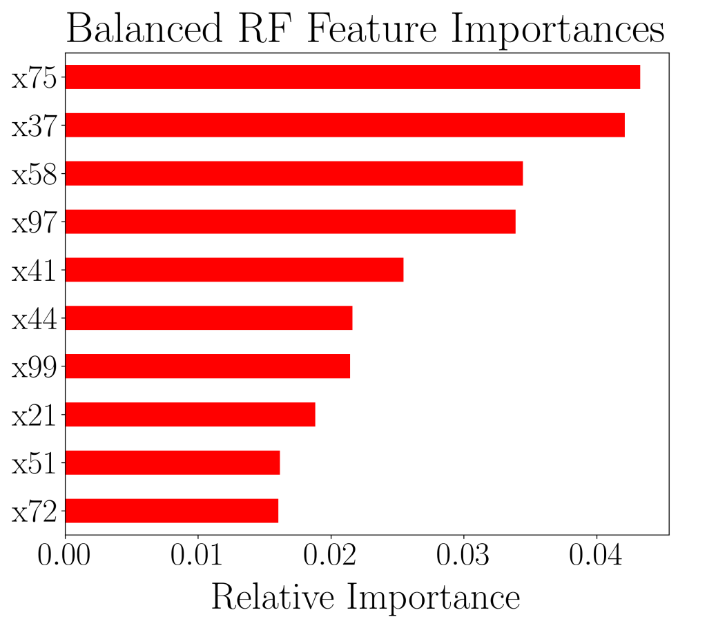
RandomForestClassifier and BalancedRandomForestClassifier.The ROC curves between the two models does not differ much and we are unable to discern the quality of the results. We then, turn to plot the top 10 most important features and notice that 7 out of 10 of the top 10 features coincide, and in fact the top 2 most important features coincide. Unfortunately, up to this point, there still isn’t enough information to distinguish the quality of the two models.
RandomForestClassifier and BalancedRandomForestClassifier.We move on to look at the confusion matrix and the classification reports provided by scikit-learn.
| Predicted | ||||
| 0 | 1 | |||
| Random Forest | Actual | 0 | 9565 | 9 |
| 1 | 1567 | 859 | ||
| Balanced Random Forest | Actual | 0 | 8700 | 874 |
| 1 | 219 | 2207 |
| Precision | Recall | F1-score | ||
| Random Forest | 0 | 0.86 | 1.00 | 0.92 |
| 1 | 0.99 | 0.35 | 0.52 | |
| Balanced Random Forest | 0 | 0.98 | 0.91 | 0.94 |
| 1 | 0.72 | 0.91 | 0.80 |
From the above analysis, we can see that the RandomForestClassifier has a very low false negative value due to its over-prediction of the majority outcome 0. The BalancedRandomForestClassifier, however, does not have this problem. Looking at precision, recall and f1-score, we see poor performance metrics for RandomForestClassifier for the minority outcome 1 in both the recall and f1-score. In contrast, the BalancedRandomForestClassifier has an overall well-rounded accuracy metric for all three of them.

In this case, precision did not manage to pinpoint the shortcomings of the RandomForestClassifier. Over-prediction of majority outcomes is not able to show up in this metric.

Recall, however, was able to pick up the discrepancies because it does not have sum of predicted conditions in its computation. Measured by the sum of real positive conditions, recall was able to single out the over-prediction of outcome 0 by the RandomForestClassifier. For the same reason, the f1-score, which is a harmonic mean between precision and recall, would have also been able to pick up the flaws of the RandomForestClassifier.

Nevertheless, besides recall and f1-score, other metrics exist for measuring performance of machine learning models on imbalanced data sets. imblearn.metrics.classification_report_imbalanced provides a classification report that further includes geometric mean and index_balanced_accuracy of the geometric mean.
| Geometric Mean | Index Balanced Accuracy | ||
| Random Forest | 0 | 0.59 | 0.38 |
| 1 | 0.59 | 0.33 | |
| Balanced Random Forest | 0 | 0.91 | 0.83 |
| 1 | 0.91 | 0.83 |
For binary classification problems, the geometric mean is calculated as the square root of the specificity multiplied by recall, and the index of balanced accuracy balances any scoring according to the imbalanced data.

We conclude this article by noting that usual accuracy metrics, such as AUC score, ROC curve, accuracy and precision may fail to reveal the shortcomings of a machine learning model’s ability to predict the minority outcome. Recall, geometric mean, and index of balanced accuracy can be favorable for imbalanced data modeling, providing a more well-rounded validation on the model’s predictive power.

Pingback: Types of Machine Learning Performance Metric and When To Use Them – Data Bay Today
Pingback: Deep Learning Neural Networks with Keras for Classification Problems – Data Bay Today