The data set we use here is a simulated data that resembles closely to real-world data, and it can be downloaded here. It requires substantial data manipulation, including cleaning, binning, imputing and one-hot encoding before the machine learning model can train on it.

Cleaning

Thorough EDA in this post revealed several spelling mistakes, and we will fix them using pandas.Dataframe.replace, where the Dataframe is df in the code.

def clean_data(df):

    # Strip units
    df.x41 = df.x41.str.strip('$')

    # Convert numeric predictor to float
    df.x41 = df.x41.astype(float)

    # Correct spelling errors in car models
    df.x34 = df.x34.replace({'chrystler':'CHRYSLER', 'mercades':'MERCEDES'}).str.upper()

    # Standardize day of week column
    df.x35 = df.x35.replace({'monday':'MON', 'tuesday':'TUE', 'wednesday':'WED', \
                             'thurday':'THR', 'thur':'THR', 'friday':'FRI'}).str.upper()

    # Standardize zeros
    df.x45 = df.x45.replace({'-0.0%':'0.0%'})

    # Standardize months column
    df.x68 = df.x68.replace({'Dev':'DEC', 'sept.':'SEP', 'January':'JAN', \
                             'July':'JUL'}).str.upper()

    # Correct spelling errors in countries
    df.x93 = df.x93.replace({'euorpe':'EUROPE'}).str.upper()
    
    return df

The function clean_data fixes all spelling mistakes in categorical predictors replacing the fixes in-place with pandas. The EDA revealed spelling errors, non-standardization in capitalization, and presence of units in the data. Paying close attention to details is certainly a pre-requisite for the data scientist.

Binning

Levels of a categorical predictor that made up less than 5% of the total observations for the column were collapsed into either: (a) another level with a similar “hit rate” on y (i.e., x45), (b) the biggest level (i.e., x36), or (c) a level that is theoretically similar (i.e., x35, x68, x93,). Minimizing the number of levels can be advantageous in CART models because high cardinality (i.e., many levels in a predictor) produces sparsely populated features after one-hot encoding and ultimately attenuates the feature importance of the original categorical predictor, making it “fade into the woodwork” in comparison to the numeric predictors.

Using the categorical predictor x34 as an example, we see that Chrysler, Nissan, Mercedes, Ford and Chervolet all contain very small counts (< 5%) and hence we bin it together with Volkswagon (which has the highest count). Binning low levels of data helps to improve accuracy of machine learning models by reducing the impact of noise and non-linearity.

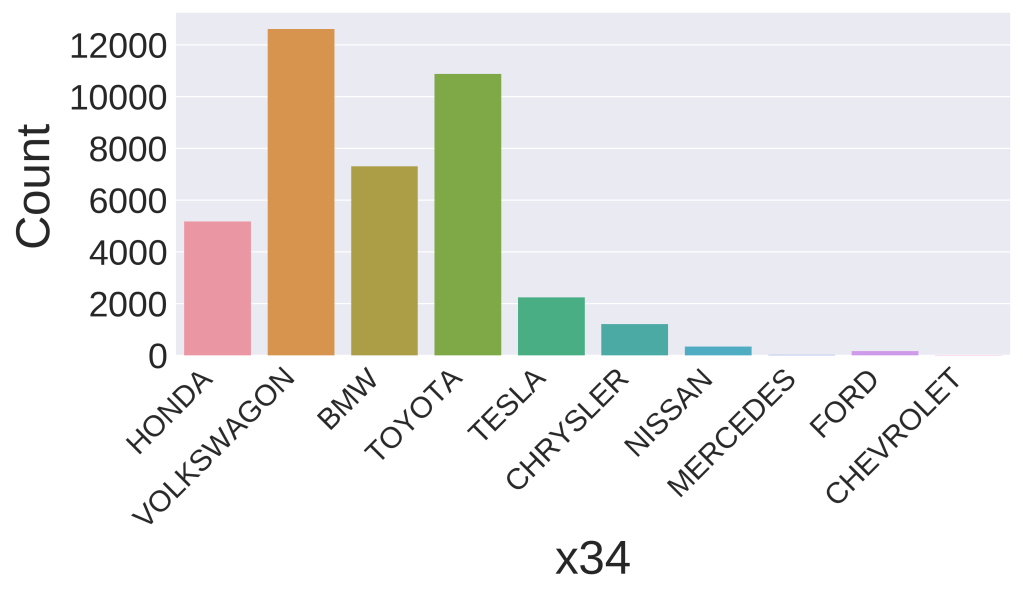
The code below shows the function which bins all the levels which are <5% to create a new categorical value.

def binning(df):

    # Binning car models (CHEVROLET, CHRYSLER, MERCEDES, FORD, NISSAN, VOLKSWAGON into OTHERS)
    df.x34 = df.x34.replace({'CHEVROLET':'OTHERS', 'CHRYSLER':'OTHERS', 'MERCEDES':'OTHERS',\
                             'FORD':'OTHERS', 'NISSAN':'OTHERS', 'VOLKSWAGON':'OTHERS'})

    # Binning day of week (beginning of week [Mon, Tues, Weds] vs. end of the week [Thurs, Fri])
    df.x35 = df.x35.replace({'MON':'M-W', 'TUE':'M-W', 'WED':'M-W', \
                             'THR':'TH-F','FRI':'TH-F'})

    # Binning percentages (y "hit rate" positively correlated with this predictor,
    # so adding small levels of predictor to neighboring levels with similar hit rates)
    df.x45 = df.x45.replace({'-0.04%':'<=-0.02%', '-0.03%':'<=-0.02%', '-0.02%':'<=-0.02%', \
                             '0.04%':'>=0.02%', '0.03%':'>=0.02%', '0.02%':'>=0.02%'})

    # Binning months (binning into seasons; winter, spring, summer, fall)
    df.x68 = df.x68.replace({'DEC':'WINTER', 'JAN':'WINTER', 'FEB':'WINTER', \
                             'MAR':'SPRING', 'APR':'SPRING', 'MAY':'SPRING', \
                             'JUN':'SUMMER', 'JUL':'SUMMER', 'AUG':'SUMMER', \
                             'SEP':'FALL', 'OCT':'FALL', 'NOV':'FALL'})

    # Binning countries (asia vs. western)
    df.x93 = df.x93.replace({'EUROPE':'WESTERN', 'AMERICA':'WESTERN'})
    
    return df

Imputation

Imputing missing data helps to prevent data from being lost due to deletion. It helps to preserve and salvage the data entries, by opting for a method deemed suitable to the data set. There exists many imputation techniques, some more advanced than others, and we generally go by the following rule of thumb:

1. Type of missing data: Determine the type of missing data (missing completely at random, missing at random, or missing not at random).
2. Imputation technique: Apply an appropriate imputation method for the type of missing data.
3. Review and revise: Revise, if necessary, the imputation technique, based on the machine learning accuracy metrics from hold-out data.

In our present case, we opted for a simple imputation technique, and apply the mode and mean substitution for categorical and numeric predictors, respectively. About 2% of cases (rows) within the current dataset contained missing values, which were spread fairly evenly among predictors. This missing data may or may not be Missing Completely at Random (MCAR), hence the decision to use imputation rather than list-wise deletion. This can be easily achieved using sklearn.impute.SimpleImputer, where the strategy (mean, mode or median) is simply an input.

One-hot Encoding

Feature engineering can play an important role in the data cleaning process to enable powerful, predictive data sets for machine learning models. Unfortunately, machine learning models are unable to make use of categorical predictors. Depending on the software used, the model usually ignores it. This can be potentially dangerous as useful information encased in these categorical predictors are thrown out without warning. The procedure of converting these categorical predictors into numeric predictors is known as one-hot encoding. To shed more light into what and how it does, we go back to predictor x34. Say for example, one of the row entries shows that x34 is a Honda, and recall that after binning, the values left in x34 are “HONDA”, “BMW”, “TOYOTA”, “TESLA” and “OTHERS”. The result of using pandas.get_dummies is as follows:

It is clear that the operation resulted in more columns being created and in fact, the number of extra columns is the number of unique values in the categorical predictor. As such, we will have to append these new columns to the dataframe using pandas.concat.

def one_hot_encoding(df):

    index = ['x34', 'x35', 'x45', 'x68', 'x93']
    for i in range(len(index)):
        df = pd.concat([df, pd.get_dummies(df[index[i]])], axis=1).drop([index[i]], axis=1)
    
    return df

And we do these for all the categorical predictors.

Output clean data set

The new, clean data set can then be written out into a csv file.

# Output clean data
    df.to_csv('clean_data.csv', index=False)

We removed the first column of indexing so that it follows the original data formatting. This clean_data.csv can be downloaded here, and we will use it in subsequent posts for training machine learning models.