
This article illustrates the use of Deep Learning, and more specifically the multilayer perceptron (MLP) for the purpose of forecasting stock prices for IBM. In a previous article, we’ve demonstrated the use of traditional time-series analysis using the ARIMA model. The results were fascinating, as we saw that the normalized mean squared error was in the fourth decimal place. With the advent of machine learning and deep learning algorithms in recent years, we would like to test these new methods with the age-old challenge of stock price forecasting. Stock price forecasting have been considered to be a challenging endeavor for a long time because both accuracy and cost (time spent on modeling) matters in this fast-paced financial data. These data are inherently stochastic processes, and are often non-stationary. Many quantitative methods exist, and some better than others. Today, we look at the use of MLP for the purpose of forecasting the open stock price for IBM.
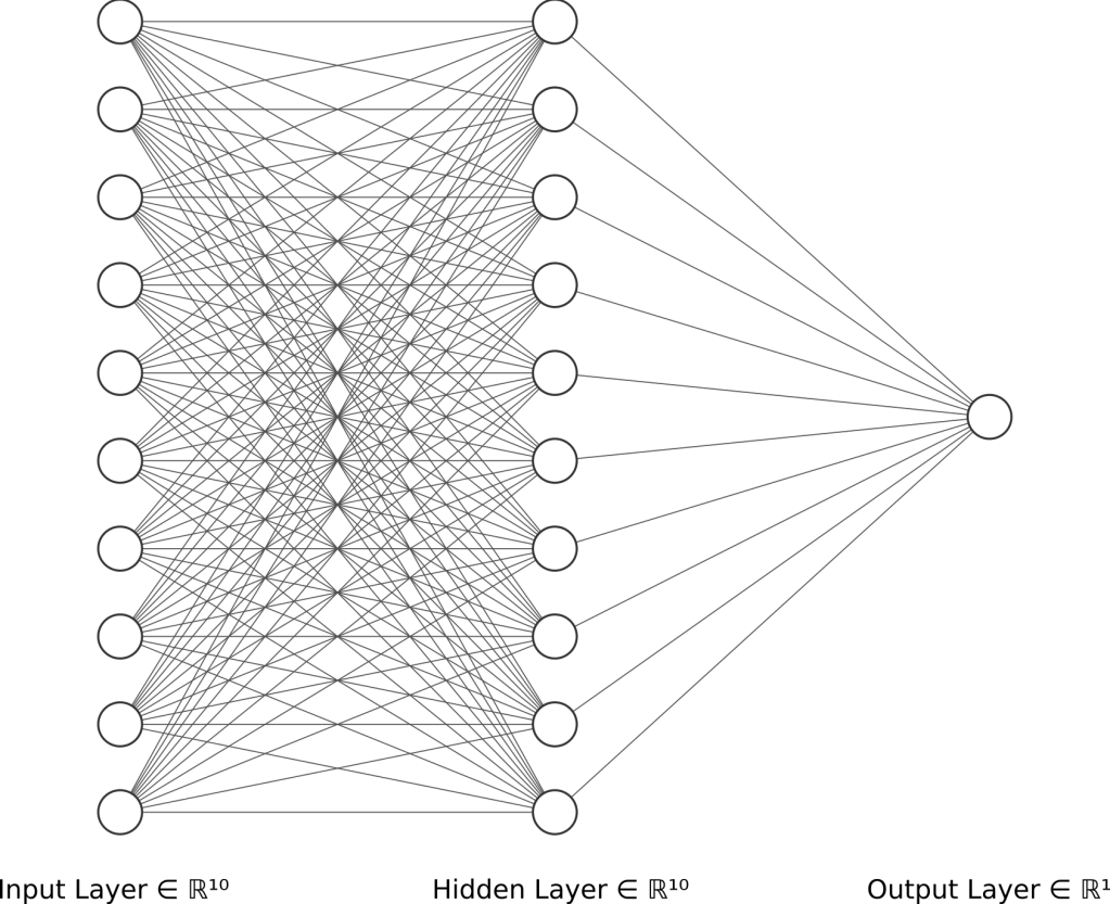
The MLP is a class of feedforward neural network composed of multiple layers of perceptrons. It typically consists of at least 3 layers of neurons: the input layer, hidden layer, and output layer. Each neuron uses a nonlinear activation function which helps in the modeling of nonlinear data. Below is an example of a neural network with three layers. In fact, this will be the exact model configuration we’ll be using for our stock price forecasting. We’ll demonstrate that this simple neural network configuration can be surprisingly accurate, even without optimizing its model parameters.
The financial data can be acquired at this Kaggle site, and more specifically in the directory “Data/Stocks/ibm.us.txt” of the downloaded folder. This set of data consist of stock prices from 1962-01-02 to 2017-11-10, and as usual we aim to split the data into 70% train set and 30% validation set in order to quantify the model’s accuracy. Since the data is a time-series, which means that it consists of one column of dates, and one column of the variable of interest, we will need to transform the time-series data into a supervised learning dataset. This is necessary because inputs for Machine Learning models have to be formatted in a way so that the algorithm can train its model parameters.
The article will be sectioned into the following:
- Data Manipulation: we demonstrate how the time-series data can be split into 70% training set and 30% validation set, and show how it can be converted for supervised machine learning purposes
- Building the Multilayer Perceptron (MLP): we explain what the MLP is, and demonstrate it with Keras, a deep learning Python library
- Model Validation: the MLP model is then validated with metrics to verify the accuracy of the model
Data Manipulation
Preprocessing of data before modeling is often dreadful, and we hope that by shedding more light into why we do them, the how will get easier. Firstly, we read the data using pandas, and the variable df is of now, a dataframe.
import pandas as pd

# Read file (only dates and open prices)
df = pd.read_csv('/data/Data/Stocks/ibm.us.txt')[['Date', 'Open']]
We then convert the prices column into a single NumPy array called dataset for later use. Assigning the type to Python default ‘float’, ensures that the array is of double precision.
# Convert to numpy
dataset = df[['Open']].values
dataset = dataset.astype('float')
The open price dataset is then split into 70% training and 30% validation (test) set. Due to the nature of time-series data, we cannot randomly select the train and test set. Hence, we pick the first 70% of data ranging from 1962-01-02 to 2001-02-05 to train the MLP model, and use them to forecast the prices between 2001-02-06 to 2017-11-10.
# Split dataset into 70% train, 30% test
train, test = dataset[0:int(len(dataset) * 0.7),:],
              dataset[int(len(dataset) * 0.7):len(dataset),:]
Next, comes the important part of converting the time-series data into usable supervised learning data. We’ll first illustrate the concepts, then introduce the coding. The original time-series data looks like the following.
| Date | Open | |
| 0 | 1997-05-16 | 1.97 |
| 1 | 1997-05-19 | 1.76 |
| 2 | 1997-05-20 | 1.73 |
| … | ||
| 5150 | 2017-11-08 | 1122.82 |
| 5151 | 2017-11-09 | 1125.96 |
| 5152 | 2017-11-10 | 1126.10 |
In supervised learning, the ML model is always trying to learn a function given some input and output. As such, the training data will have to be in a similar form, where the function f takes in an input x, and gives out an output y.
f(x) = y
Hence, one excellent way to transform it would be to let x be values at time t, and y be values at time t+1. The MLP model will be building the function f that gives the predictions! The transformed data will look like the following.
| x | y |
| 1.97 | 1.76 |
| 1.76 | 1.73 |
| … | … |
| 1122.82 | 1125.96 |
| 1125.96 | 1126.10 |
The code that does this transformation is given below.
def time_series_to_supervised_learning(dataset, step=1):
    X, y = [], []
    for i in range(len(dataset)-step-1):
        a = dataset[i:(i+step), 0]
        X.append(a)
        y.append(dataset[i + step, 0])
    return np.array(X), np.array(y)
step refers to the number of prior time steps that will be used for predicting the next one. If step=3, then the prediction for time t+1 depends on time t, t-1, and t-2. As such, the resulting supervised learning dataset will have 3 columns of x, i.e. t-2, t-1, t, and 1 column of y, i.e. t+1.
With this function, we convert our train and test dataset accordingly with step=1.
# Reshape such that X=t and Y=t+1
X_train, y_train = time_series_to_supervised_learning(train, step=1)
X_test, y_test = time_series_to_supervised_learning(test, step=1)
And now, our data is ready for modeling!
Building the Multilayer Perceptron (MLP)
First, we import libraries and functions that’ll be needed.
import math as ma
from keras.layers import Dense
from keras.models import Sequential
from sklearn.metrics import mean_squared_error
We’ll be using a dense, sequential neural network, using the normalized mean squared error as the accuracy metric. We normalize the mean squared error by the mean of the values so that the error metric ranges between 0 and 1, with 1 being absolutely inaccurate, and 0 having no errors.
The MLP is instantiated and given an input layer of 10 neurons, a hidden layer with 10 neurons, and a single output neuron. ReLU is chosen as the nonlinear activation function, because of its robustness compared to the sigmoid and tanh.
# Instantiate Multilayer Perceptron (MLP) model
model = Sequential()

# Input layer
model.add(Dense(10, activation='relu', input_dim=step))
# Hidden layer
model.add(Dense(10, activation='relu'))
# Output layer
model.add(Dense(1))
This is followed by a simple fitting of the model, with the loss function set as the mean squared error, choosing the adam optimizer. The adam optimizer has been proven to be more accurate and robust than the stochastic gradient descent, requiring little to no tweaking of parameters.
# Compile model
model.compile(loss='mean_squared_error', optimizer='adam')

# Fit model
model.fit(X_train, y_train, epochs=10, batch_size=3, verbose=2)

# Train model
y_train_pred = model.predict(X_train)

# Test model
y_test_pred = model.predict(X_test)
We calculate the predictions for the training and test set, so that we can check for over-fitting. In the scenario where the model over-fits, the accuracy metric for the train set will be a lot higher than the test set.
Model Validation
The model is now validated against the actual data. The predicted data for the validation (test) set is plotted over the actual data.
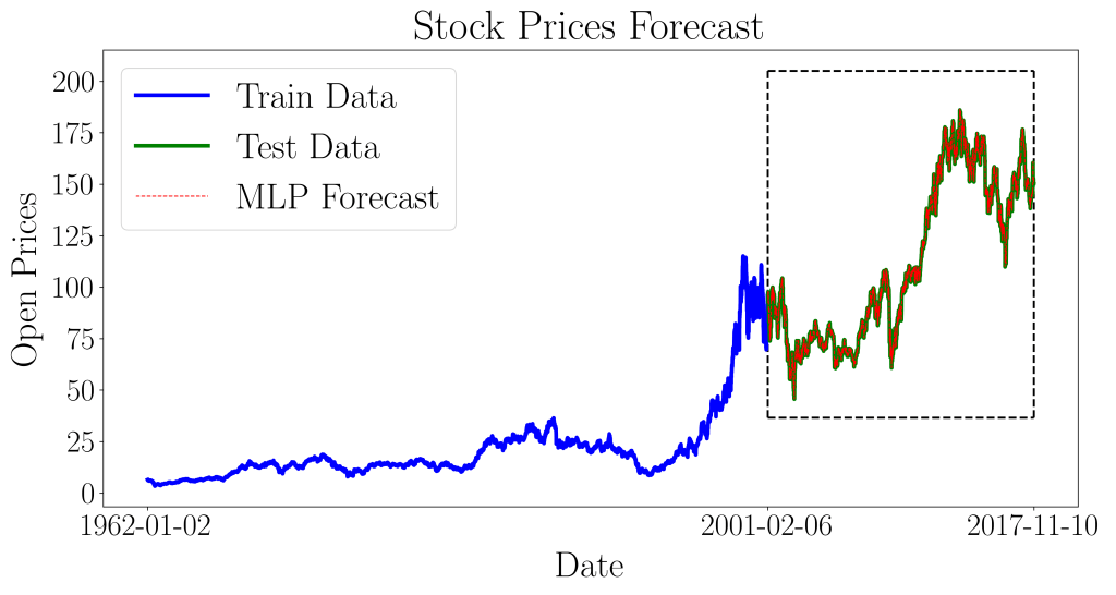
We now zoom into the box region for a better view of its prediction accuracy.
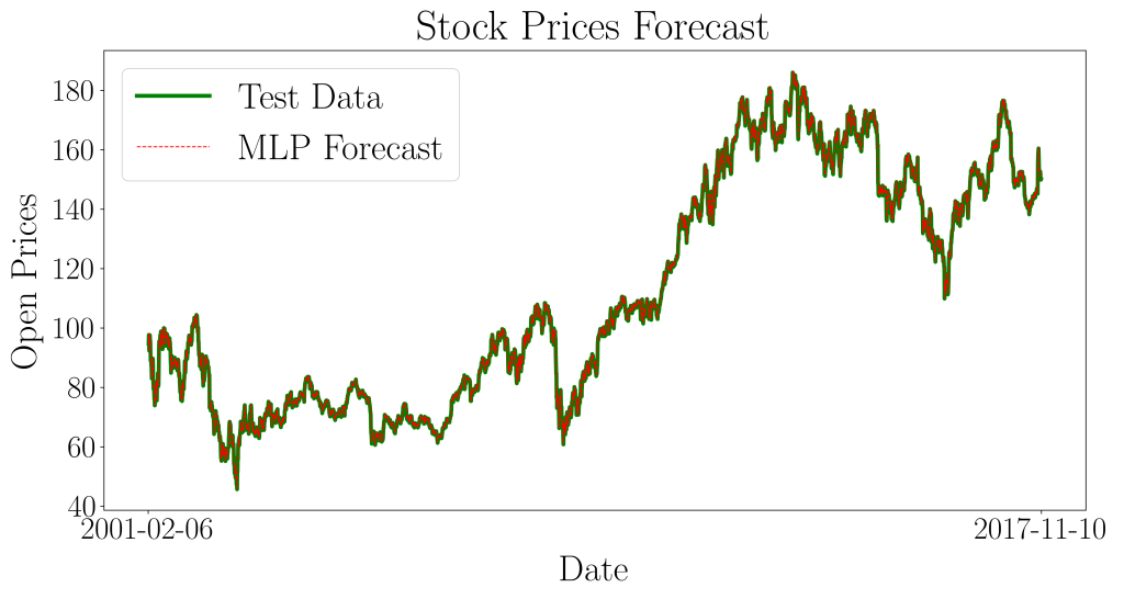
The resulting normalized mean squared error for the training data is 0.00023370, and the normalized mean squared error for the validation (test) set is 0.00059423. The two results are of the same order of magnitude, and hence the model is well-fitted. Notice that the error for the test set is in the fourth decimal place!
This concludes our multilayer perceptron demonstration for forecasting the ever so challenging data – stock prices. In this article, we showcased an alternative method of modeling time-series data using Deep Learning algorithms, rather than traditional statistical methods such as ARIMA models. We also demonstrated how time-series data can be transformed into supervised learning datasets, for the purpose of training the model with MLP. We hope you enjoyed this article and hopefully you can also be creative with your data, exploring new ways of applying machine learning in everyday life.
