
Convolutional neural network (CNN) is a class of deep learning neutral network which is most popularly used for analyzing images. The term convolution is a mathematical operation on two functions, creating a third function which expresses how each of the input functions shape each other. Similarly, in CNNs a chosen kernel convolves with the data image and produces data that allows the model to identify whether a certain block of pixels represent an edge, a color change, etc. Data image for CNNs are of the following format in Keras.

In Keras, this would be a four index NumPy array. The first index contains the number of images, second index is the number of pixels for the width, third index is number of pixels for the height, and final index refers to the red, green, or blue. For a fully colored image data, the final index will have a value of 3.
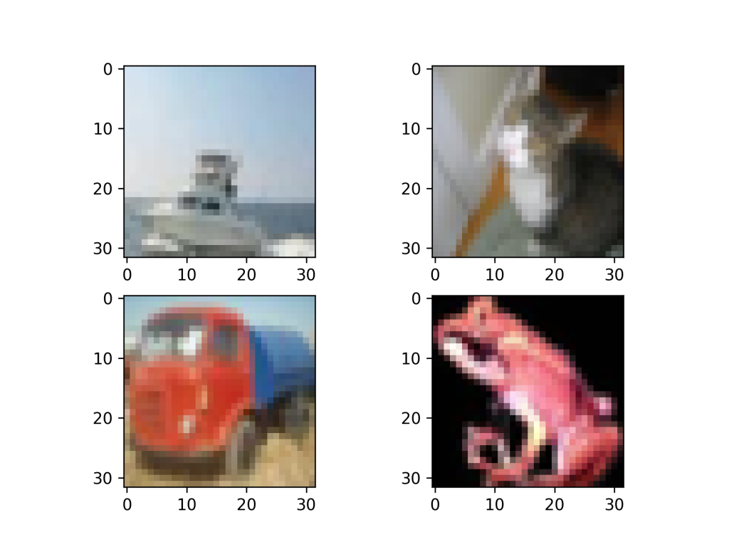
In this article, we will introduce the concepts of CNN with a demonstration. After all, the best way to learn something is to simply do it! We will use Keras to implement a CNN multiclass image classifier, using a very challenging dataset CIFAR-10. This data set can be downloaded directly from the Keras package, and we will demonstrate how to do it below. The CIFAR-10 contains 50,000 training data and 10,000 validation data. It has images of various objects, and the task is to correctly label those images under 10 different classes (ranging from class 0 – 9) in the following order: airplane, automobile, bird, cat, deer, dog, frog, horse, ship, and truck. This data set has been used in a Kaggle competition, and a classification accuracy of >90% is considered to be extremely good performance!
Our CNN demonstration will be as follows:
- Data Loading: We will load the data from Keras and observe the format and data type of the images.
- Data Format Conversion: The data is then converted to a format that is compatible with Keras inputs for model training.
- Model Building and Training: A baseline CNN model is built and trained with the data set.
- Model Validation: We validate the CNN model by applying it to the validation set, check of various performance metrics, and discuss areas of improvement for better accuracy.
Data Loading
The data is loaded from keras.datasets and the outputs are conveniently separated into train and test sets. If one examines the shape of the train or test set, with X_train.shape and X_test.shape, we will see that the image data has four indices and is stored in the manner as explained previously, with 50,000 training data and 10,000 validation data.
def read_data():
    from keras.datasets import cifar10

    # Load data into predictors 'X' and outcome 'y'
    (X_train, y_train), (X_test, y_test) = cifar10.load_data()

    return X_train, X_test, y_train, y_test
Data Format Conversion
The critical first step, would be to print out and observe the data type and structure of the predictors X and outcomes y. The predictors are seen to be of integer type, having pixel values ranging from 0 to 255, for each of the red, blue, and green colors. For better classification performance, one common practice is to normalize these values such that the range between [0, 1]. It is, important to remember to convert the predictor arrays to floats first, before the division to avoid erroneous integer results.
def convert_data_format(X_train, X_test, y_train, y_test):
    from keras.utils import np_utils

    # Convert integer arrays to float and normalize to [0, 1]
    X_train = X_train.astype(float)/np.max(X_train)
    X_test  = X_test.astype(float)/np.max(X_test)

    # One-hot encoding for outcome (10 classes)
    y_train = np_utils.to_categorical(y_train).astype(int)
    y_test = np_utils.to_categorical(y_test).astype(int)

    return X_train, X_test, y_train, y_test
The classification outcome variable y is also seen to have a size of 10,000 by 1, with values such as
[3, 8, 8, … 5, 1, 7].
We apply one-hot encoding using np_utils from Keras such that the new array is of size 10,000 by 10, and the same array looks like the following.
| Class 0 | Class 1 | Class 2 | Class 3 | Class 4 | Class 5 | Class 6 | Class 7 | Class 8 | Class 9 |
| 0 | 0 | 0 | 1 | 0 | 0 | 0 | 0 | 0 | 0 |
| 0 | 0 | 0 | 0 | 0 | 0 | 0 | 0 | 1 | 0 |
| 0 | 0 | 0 | 0 | 0 | 0 | 0 | 0 | 1 | 0 |
| … | |||||||||
| 0 | 0 | 0 | 0 | 0 | 1 | 0 | 0 | 0 | 0 |
| 0 | 1 | 0 | 0 | 0 | 0 | 0 | 0 | 0 | 0 |
| 0 | 0 | 0 | 0 | 0 | 0 | 0 | 1 | 0 | 0 |
Model Building and Training
This section will be broken down into smaller subsections for a clearer overview of how to implement the CNN model, and why we chose certain parameters in our modeling process.
Initialize the model
The model we picked is a sequential one, which simply means a linear stack of neural networks. The other option that Keras provides is Model (functional API). This is mainly for building complex networks with multiple inputs and outputs.
from keras.models import Sequential
# Initialize sequential model
model = Sequential()
Adding the neural network layers
The first layer is the input layer, and we have chosen to pick a 3 by 3 convolution kernel. This convolution kernel will do a convolution with the image data and pick up features in the data that will help in our classification training process. The padding here, refers to padding the input data with zeros on all sides such that the output data has the same size. The default in Keras is without padding, and hence the output data will be of a different size, than the input. ReLU is chosen as the activation function, because it results in better gradient propagation than the sigmoid function, and it is also computationally more efficient.
from keras.layers import Dense, Flatten
from keras.layers.convolutional import Conv2D

# Number of pixels, colors, classes
n_cols = X_train.shape[1]; n_color = X_train.shape[3]; n_class = y_train.shape[1]


# Input layer
model.add(Conv2D(n_cols, (3, 3), input_shape=(n_cols, n_cols, n_color), padding='same', activation='relu', kernel_constraint=maxnorm(3)))

# First hidden layer
model.add(Conv2D(n_cols, (3, 3), activation='relu', padding='same', kernel_constraint=maxnorm(3)))

# Second hidden layer
model.add(Flatten())
model.add(Dense(500, activation='relu', kernel_constraint=maxnorm(3)))

# Output layer
model.add(Dense(n_class, activation='softmax'))
In the first hidden layer, the input_shape is no longer needed since it only applies to the input layer. We do the same convolution with a 3 by 3 kernel in this layer, giving it the same number of nodes as the number of predictors. The padding is also set to “same” such that the output retains its size. In the second hidden layer, however, we have decided to switch back to a densely connected neural network and this requires us to call the function Flatten. This is necessary before switching back to dense networks, to preserve weight ordering when switching a model from one data format to another. We apply the ReLU activation function in this layer as well, and this time we increased the number of nodes to 500. For the final output layer, we restricted the number of nodes such that it is the same as the number of classifications. The softmax activation function is used in the last layer because it works well with multiclass classification problems. It outputs the probability of each data belonging to each class, allowing us to easily classify the data based on a threshold (probability ≥ 0.5). The kernel_constraint=maxnorm(3) means that if at any time, the L2-norm of the network weights exceeds the value 3, it rescales the weight matrix by a factor that reduces the L2-norm to 3. This has been proven to prevent overfitting in deep learning neural networks (Srivastava, et al., 2014).
Compiling the Model
The model is then compiled with the choice of optimizer, loss function and performance metric. The optimizer is chosen as ‘adam’, because it is computationally more efficient and performs much better than classical stochastic gradient descent. It is an adapted algorithm from stochastic gradient descent which updates its network weights as the training proceeds, allowing for better tuning of the parameters and hence better model performance. Classical stochastic descent unfortunately keeps all its learning weights constant throughout the training process. The loss function is chosen as categorical_crossentropy, and this loss function is well-suited for multiclass classification problems. We also choose the performance metric as classification accuracy for validating our model’s predictive power.
# Compile model
model.compile(optimizer='adam',
              loss='categorical_crossentropy',
              metrics=['accuracy'])
Checkpointing in Keras
Checkpointing allows the user to save the weights of the best model, as determined by the chosen performance metric, during the training process. In the code below, we save the network weights of the best model in a file called “best_model.h5”. This file can later be loaded using the Keras function keras.models.load_model, and the neural network can be used immediately without the need to got through training again.
# This checkpoint object will store the model parameters in the file "best_model.h5"
checkpoint = ModelCheckpoint('data/best_model.h5', monitor='val_loss', mode='min', save_best_only=True)

# Store in a list to be used during training
callbacks_list = [checkpoint]
monitor='val_loss', mode='min' means that the “best model” is one which minimizes the loss value on the validation set. The callbacks_list will be fed as an input to model.fit during training, for storing the parameters (network weights) of the best model.
Model Training
# Fit the model
history = model.fit(X_train, y_train, validation_data=(X_test, y_test), epochs=10, callbacks=callbacks_list)
The CNN model is trained with the training data set, and the validation set is also provided so that we can monitor the validation accuracy score of the model as the training progresses. The input callbacks=callbacks_list allows the most optimal weights to be stored externally and can be loaded back up into the code for other uses.
Lastly, we can call model.summary() for a print out of the model’s layers and parameters, giving a summary of the CNN model.
| Layer (type) | Output Shape | Param # |
| conv2d_1 (Conv2D) | (None, 32, 32, 32) | 896 |
| conv2d_2 (Conv2D) | (None, 32, 32, 32) | 9248 |
| flatten_1 (Flatten) | (None, 32768) | 0 |
| dense_1 (Dense) | (None, 500) | 16384500 |
| dense_2 (Dense) | (None, 10) | 5010 |
Model Validation
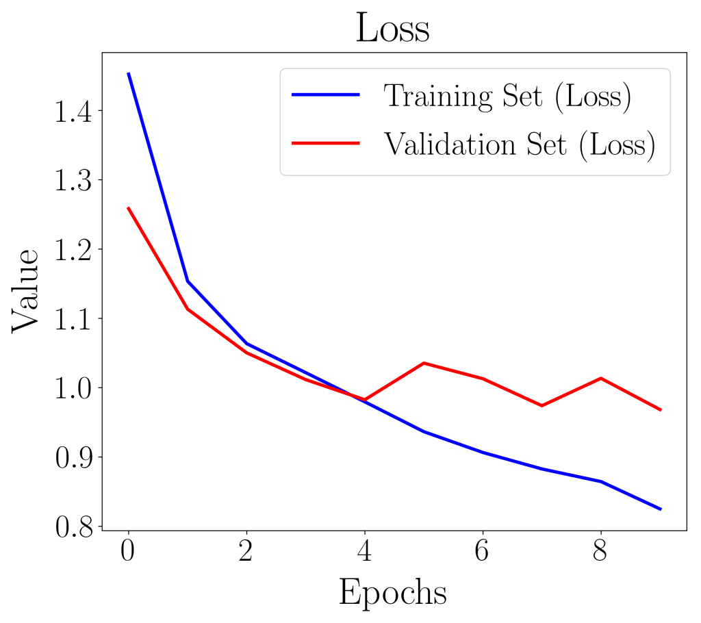
The loss and accuracy plots showed signs of maxnorm rescaling the weight matrix to prevent overfitting of the model. For instance, the validation loss curve increased at the 5th epoch, and went down again on the 6th, and increased again at the 8th. The maxnorm can be considered as a form of regularization where weights with higher weight are more heavily penalized. This shows the importance of understanding the input parameters for the CNN model.
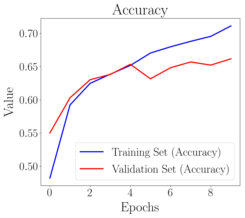
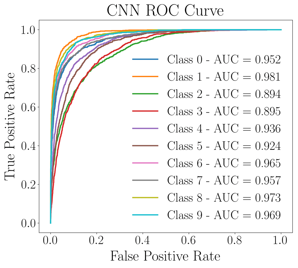
The ROC curve as well as the AUC score, did pretty well despite poor accuracy performance of on 0.796 training set and 0.662 on validation set. The AUC score in this case, did not reveal much regarding the nature of the model’s predictive power.
| Precision | Recall | Specificity | F1-score | Geometric Mean | |
| Class 0 | 0.24 | 0.85 | 0.70 | 0.37 | 0.77 |
| Class 1 | 0.75 | 0.83 | 0.97 | 0.79 | 0.90 |
| Class 2 | 0.69 | 0.32 | 0.98 | 0.44 | 0.56 |
| Class 3 | 0.65 | 0.20 | 0.99 | 0.30 | 0.44 |
| Class 4 | 0.75 | 0.45 | 0.98 | 0.56 | 0.66 |
| Class 5 | 0.66 | 0.42 | 0.98 | 0.52 | 0.64 |
| Class 6 | 0.75 | 0.71 | 0.97 | 0.73 | 0.83 |
| Class 7 | 0.81 | 0.64 | 0.98 | 0.71 | 0.79 |
| Class 8 | 0.87 | 0.65 | 0.99 | 0.74 | 0.80 |
| Class 9 | 0.83 | 0.67 | 0.98 | 0.74 | 0.81 |
Classification report from imbalanced-learn reveals that the model had more trouble classifying some class. For instance, class 0 (airplane), class 2 (bird), and class 3 (cat) had poor performance metrics on F1 score. Class 0 even had 0.24 for precision, revealing poor accuracy performance.
Overall, this is a challenging data set that requires a much deeper neural network, and fine tuning in order to perform well. We have achieved a validation accuracy score of 66% using just 4 neural network layers, and no fine tuning! This article has served its purpose well, building and explaining the workings of a convolutional neural network. Hopefully this challenging data set will pique your interest enough to try out more rigorous CNN models!
