
Selecting the appropriate machine learning model for the data set requires knowledge and insights about the data acquired from the EDA stage. The clean data used for this exercise can be downloaded here and the post on how we cleaned this data is here. In our bivariate EDA, we learned that there isn’t strong correlation between any two predictors within the data set. As such, ensemble learning CART models which are resistant to noise, would perform well under such conditions. For this exercise, we will choose 2 CART models which are fundamentally disparate in their algorithms:
- Random forest classifier: An ensemble learning method where predictors are constructed independently, consisting of a large number of decision trees. The classification is based on the mean prediction of the individual trees.
- Gradient boosting classifier: An ensemble learning method where predictors are constructed sequentially, consisting of a large number of decision trees, each of which produces output based on minimizing the residual error of its predecessor.
It would be truly interesting to compare and contrast these 2 algorithms in terms of performance and cost. To our understanding, such direct comparisons are rare, and we think it would be valuable to compare these methods side-by-side on this challenging (imbalanced) data set. For both machine learning models, we will employ the same steps for building and verifying the model.
- Data Manipulation: split data into 70% train and 30% test, as hold-out data.
- Grid Search: Use grid search to find the best parameters for the model, using a 5-fold cross-validation and AUC score as the accuracy metric.
- Important Features: Find the top 10 most important features (out of 100 predictors) that has the most predictive power in the model.
- Model Validation: Test the model on the 30% hold-out data to validate the accuracy of model using confusion matrix, AUC score, etc.
Data manipulation
The data manipulation step will be the same for both models. First, we import relevant Python packages and read the csv file using pandas.
def read_data():
    # Read csv file
    df = pd.read_csv('clean_data.csv')

    # Transform data into predictors 'X' and outcome 'y'
    X = df.drop('y', axis=1).values
    y = df['y'].values

    return df, X, y
In the code, we let X contain the predictors and y contain the outcome. We store them separately since the machine learning model in sklearn expects inputs as such.
Next, we split the data into 70% training set and 30% test set using train_test_split from sklearn.model_selection.
def split_data(X, y):
    SEED = 100

    # Split dataset into 70% train, 30% test
    X_train, X_test, y_train, y_test = train_test_split(X, y,
                                                    test_size=0.3,
                                                    stratify=y,
                                                    random_state=SEED)
    return X_train, X_test, y_train, y_test
The seed number is set as a constant, so that the results are reproducible in separate runs. The Python function split_data takes in the predictors and outcome, splits the data set, and returns the training and testing set separately for the predictors and outcome.
Grid Search
Now, we’re able to select the “best” hyperparameters using GridSearchCV from sklearn.model_selection. GridSearchCV tests rigorously for all combinations of hyperparameters, using the k-fold cross-validation to decide the best model parameters via the criterion provided (e.g. accuracy score, AUC score, etc). In scikit-learn, even though models have default hyperparameters, these are not optimal for all problems. Hyperparameters should be tuned for each dataset in order to attain the optimal model. In this analysis, the grid search cross validation method was adopted due to its rigor and comprehensiveness. For each model, the grid search uses every combination of hyperparameter values in the grid with a 5−fold cross validation. The best model is the one which attains the best cross-validation score (in our case, highest ROC-AUC score).
Using the random forest classifier as an example, the code below first instantiates the random forest classifier, and create a grid of hyperparameters using Python dictionary. The code then instantiates the grid search function by passing the random forest classifier (rf) , the grid of parameters (params_rf), and the scoring criterion (roc_auc). Setting the input parameters n_jobs=-1 allows the sklearn module to use all available CPUs in your machine.
def initiate_gridsearch():

    # Instantiate random forest classifier 'rf'
    rf = RandomForestClassifier(random_state=SEED)

    # Define the grid of hyperparameters 'params_rf'
    params_rf = {'n_estimators': [100, 200],
                 'max_depth': [4, 8, 12],
                 'min_samples_leaf': [0.001, 0.002, 0.003, 0.004, 0.005]}

    # Instantiate a 5-fold CV grid search object 'grid_rf'
    grid_rf = GridSearchCV(estimator=rf,
                           param_grid=params_rf,
                           scoring='roc_auc',
                           cv = 5,
                           n_jobs=-1)
    return grid_rf
grid_rf which contains all the information about the grid search can then be trained with the training data set and extract the best model with the most optimized hyperparameters that has the highest AUC score.
def gridsearch(grid_rf, X_train, y_train):

    # Fit grid_rf to the training set
    grid_rf.fit(X_train, y_train)

    # Extract best model
    best_model = grid_rf.best_estimator_

    print('Best AUC score: %0.8f'%grid_rf.best_score_)
    print('Best parameters: ', grid_rf.best_params_)
    return best_model
Similar work is done for the gradient boosting classifier. The only difference is that the gradient boosting classifier is instantiated, instead of the random forest classifier. This code is versatile, robust and modular. It works with any user chosen classifier and minimal changes is needed for a different machine learning model.
Grid Search: Model I – Random Forest Classifier
Hyperparameters grid:
n_estimators(number of trees in forest) = [100, 200].-
max_depth(maximum depth of each tree) = [4, 8, 12]. -
min_samples_leaf(minimum number of samples in a leaf node) = [0.001, 0.002, 0.003, 0.004, 0.005].
The best parameters chosen by the grid search cross-validation in this case are n_estimators: 200, max_depth: 8, min_samples_leaf: 0.001, attaining a mean CV AUC score (train set) of 0.967.
Grid Search: Model II – Gradient Boosting Classifier
Hyperparameters grid:
n_estimators(number of trees in forest) = [100, 200].-
max_depth(maximum depth of each tree) = [4, 8, 12]. -
min_samples_leaf(minimum number of samples in a leaf node) = [0.001, 0.002, 0.003, 0.004, 0.005].
The best parameters chosen by the grid search cross-validation in this case are n_estimators: 200, max_depth: 12, min_samples_leaf: 0.005, attaining a mean CV AUC score (train set) of 0.987.
Important Features
We can plot out the respective model’s top 10 most important features with highest predictive power by doing the following.
importances_rf = pd.Series(best_model.feature_importances_, index=df.columns[:-1])
sorted_importances_rf = importances_rf.sort_values()[-10:]
sorted_importances_rf.plot(kind='barh', color='red')
best_model is the “best model” chosen by GridSearchCV. This allows us to compare and contrast between top 10 most important features between random forest classifier and gradient boosting classifier.
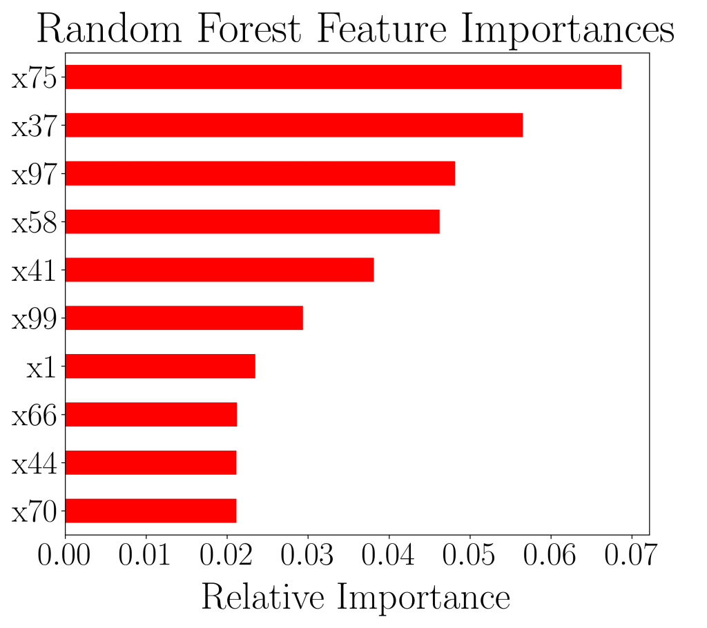
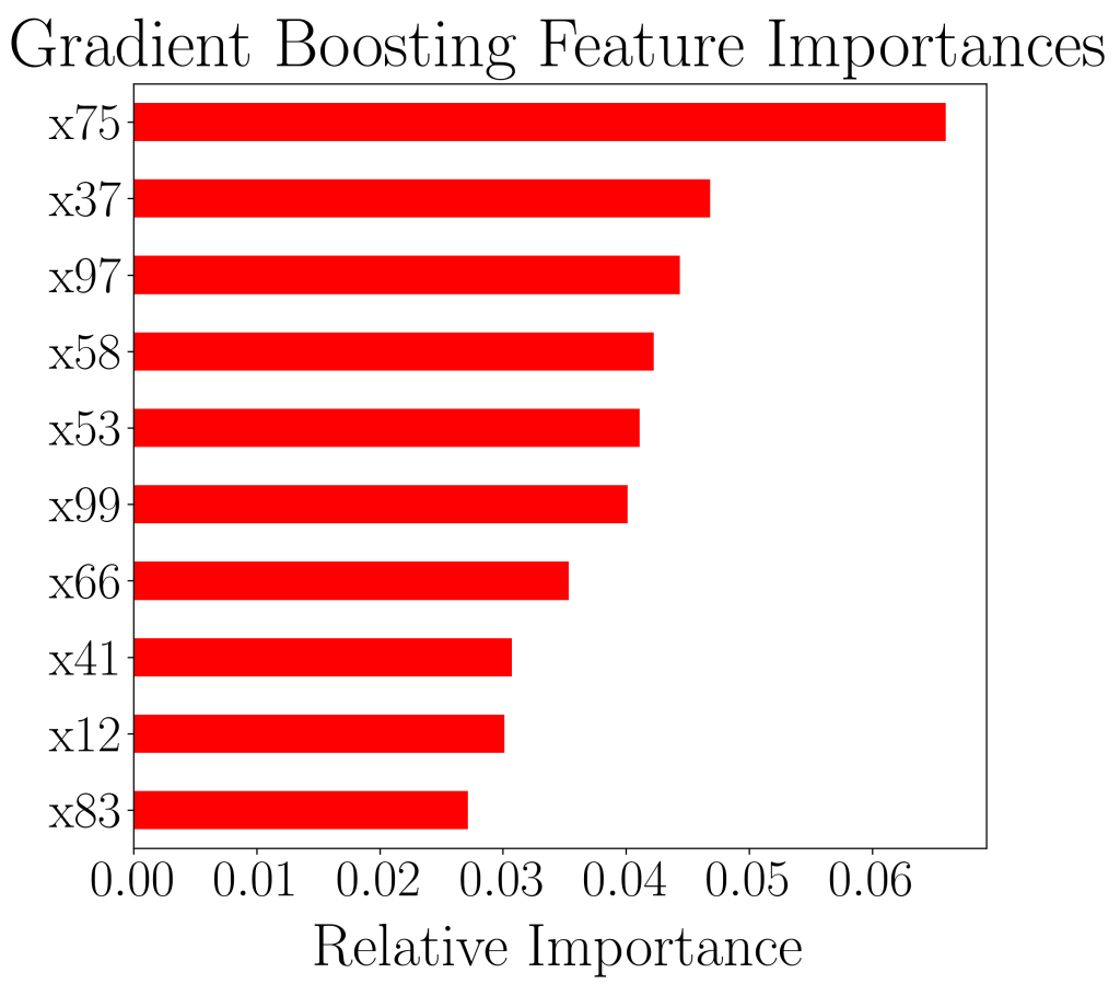
We see that in the plots above, the top 4 most predictive features (x75, x37, x97 and x58) are the same for both models. In fact, 8 out of 10 features appeared in both lists. This is encouraging, as it gives confidence on the quality of both machine learning models.
Model Validation
After the grid search cross validation has found the “best model”, it is critical to check the model and evaluate its performance. To prevent over-fitting, the training dataset was split: 70% train and 30% validation (hold-out). A model that is not over-fitted would have the cross-validation AUC score ≈ equal to the AUC score of validation set. In order for the model to be well-tested, the 5-fold cross validation was used on the training set and the mean AUC score was taken.
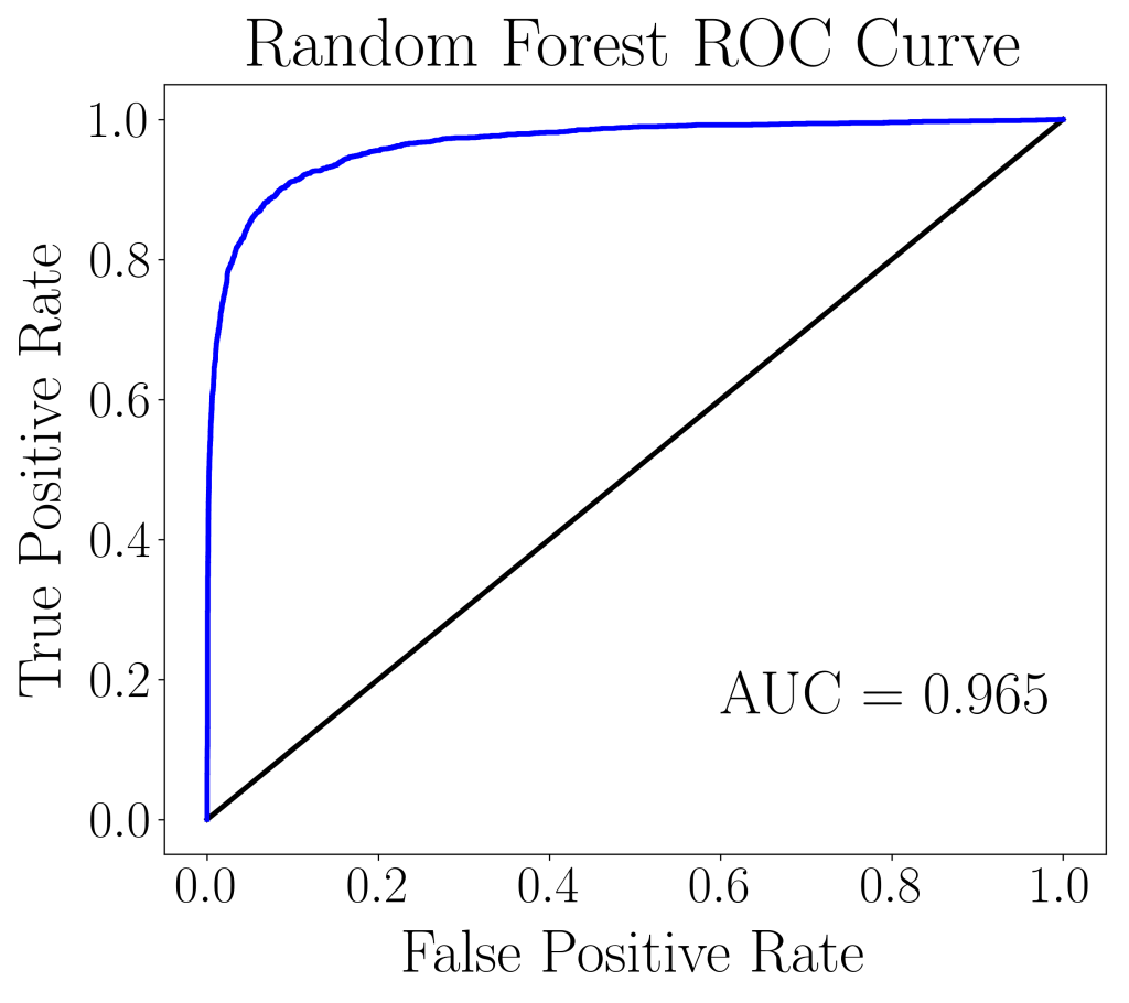
Model Validation: Model I – Random Forest Classifier
| Data set | AUC score |
| Train set (5-fold CV) | 0.967 |
| Validation/Hold-out set | 0.965 |
From the table, it is evident that the AUC scores between the train set and validation set are approximately the same. Hence, we have reason to believe that the model is well-trained with the hyperparameters chosen by the grid search cross-validation. The confusion matrix is shown below.
| Predicted | |||
| 0 | 1 | ||
| Actual | 0 | 9569 | 5 |
| 1 | 2030 | 396 |
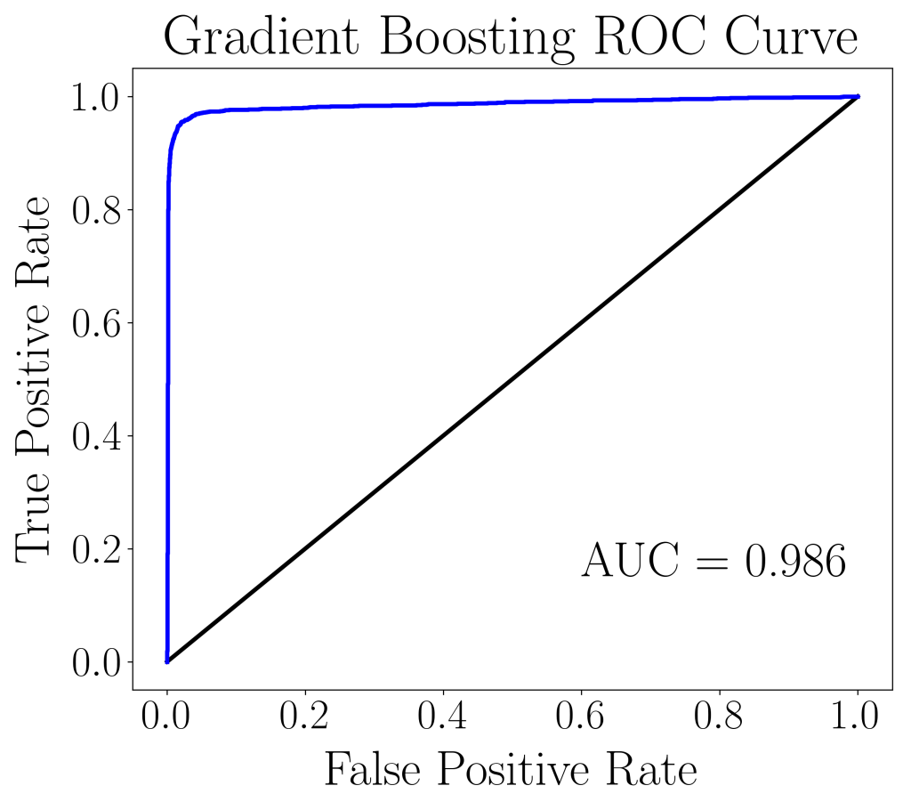
Model Validation: Model II – Gradient Boosting Classifier
| Data set | AUC score |
| Train set (5-fold CV) | 0.987 |
| Validation/Hold-out set | 0.986 |
In the table, we see that the AUC score from the 5-fold cross validation train set is indeed approximately the same as the validation set score. Hence, the model is not over-fitting and this gives us confidence to apply the trained model on real data sets. The confusion matrix is shown below.
| Predicted | |||
| 0 | 1 | ||
| Actual | 0 | 9541 | 33 |
| 1 | 287 | 2139 |
Random Forest Classifier vs. Gradient Boosting Classifier
Based on the machine learning models, we would like to compare and contrast the results obtained. We first give a summary of the two different models, then compare the performance (AUC score) as well as computational costs.
| Random Forest Classifier | Gradient Boosting Classifier | |
| Summary | An ensemble learning method where predictors are constructed independently, consisting of a large number of decision trees. The classification is based on the mean prediction of the individual trees. | An ensemble learning method where predictors are constructed sequentially, consisting of a large number of decision trees, each of which produces output based on minimizing the residual error of its predecessor. |
| Pros | 1. Faster computation due to easy parallelization. Prediction models are built independent of one another. ( scikit-learn allows parallelization with option n_jobs=-1) | 1. More optimal for predicting imbalanced outcomes (i.e., in the current case where 80% of outcomes are 0, and only 20% are 1). |
| 2. Faster hyperparameter tuning using grid search cross validation. | 2. Slightly higher AUC score on validation (hold-out) data set compared to Random Forest model. | |
| Cons | 1. Slightly lower AUC score for validation (hold-out) dataset compared to Gradient Boosting model. | 1. Slower computation and hyperparameter tuning (by grid search cross-validation), due to the sequential nature of the algorithm. |
| 2. Higher false negative rate in its predictions for validation (hold-out) data compared to Gradient Boosting model. | 2. More prone to over-fitting, which may produce less accurate predictions in the test data. |
Comparison between the predictions of the 2 models on the validation set is made below. The table shows that much of the predictions made by the two models agree with each other (diagonal entries), but the random forest classifier appears to over predict the number of 0 outcomes compared to the gradient boosting classifier. This is indicative that random forests are less robust for predicting imbalanced data.
| Gradient | |||
| 0 | 1 | ||
| Forest | 0 | 9828 | 1771 |
| 1 | 0 | 401 |

