
Sentiment analysis, sometimes also known as emotion AI or opinion mining, refers to the use of natural language processing (NLP) to systematically identify, extract, and quantify subjective information. The ability to mine information from textual data can provide valuable details that can be critical to businesses. Say for instance, customers of Amazon often leave a one to five star rating based on how much they like or dislike the product. However, such a rating system does not allow Amazon or the business owner to understand what exactly do customers like or dislike about the product. The use of NLP coupled with machine learning techniques can potentially help solve this problem without having a human painstakingly read through all the reviews. Using advanced NLP such as sentiment analysis can provide us with three insights:
- Opinion/emotion: It allows us to know the polarity (e.g. positive, neutral, negative) as well as emotion (e.g. joy, anger, disgust, etc) of the given statement.
- Subject: Tells us what is being talked about.
- Opinion holder (entity): Tells us who is giving that statement.
All these are critical parts of sentiment analysis, and are widely used in brand monitoring, customer service, product analytics, and market research and analysis.
For this reason, in today’s article, we are giving a demonstration on how to conduct sentiment analysis. We’ll be conducting sentiment analysis on 7501 IMDB reviews to build a machine learning model which can then classify reviews as positive or negative. The sample data can be downloaded here. This article will be broken down into the following sections.
- Natural Language Processing (NLP): We introduce main concepts of NLP, explaining tokenization, granularity, transforming text to numeric values using Bag-of-Words or the Tfidf (term frequency inverse document frequency) method, etc. All concepts will be illustrated with coding demonstrations using the IMDB dataset.
- Data Manipulation: We split the data into 70% training and 30% validation set, so that we can validate the model’s accuracy later on.
- Building the Machine Learning Model: In this case, we will be using the random forest classifier to classify the movie reviews as positive or negative.
- Validating the Machine Learning Model: We use various accuracy metrics such as precision, F1 score, AUC score, etc to check that our machine learning model is indeed well-trained and can be easily generalized to other datasets.
Natural Language Processing (NLP)
NLP is an amalgamation of AI, computer science, and linguistics, concerned with the use of computers to process large amounts of textual (or natural language) data. For this article, we use the Natural Language Toolkit (NLTK) for processing our data, pandas to manipulate data frames, and scikit-learn for our machine learning models. First we import python libraries concerned with this pre-processing step.
from nltk import word_tokenize
from sklearn.feature_extraction.text import TfidfVectorizer, ENGLISH_STOP_WORDS
word_tokenize will split up a sentence into its words and punctuations. For instance,
sentence = "Hello everyone! Good morning!"
print(nltk.word_tokenize(sentence))
will print the following output
['Hello', 'everyone', '!', 'Good', 'morning', '!']
Punctuations are not removed in word tokenizing because they can potentially provide very useful information. For instance, a movie review could potentially be associated as having an angry emotion because it has many exclamation marks.
We first read the data file ‘IMDB.csv’ and tokenize it.
# Read csv file
df = pd.read_csv('data/IMDB.csv')

# View the first 5 rows of data
print(df.head())

# Tokenize each item in the review column
word_tokens = [word_tokenize(review) for review in df.review]
The dataset looks like the following.
| review | label |
| SNL is pretty funny but people who say this is… | 0 |
| “Creep” is a new horror film that, without a d… | 1 |
| Ernst Lubitsch’s contribution to the American … | 1 |
| I have to say I am really surprised at the hig… | 0 |
| me and my sister have right now watch that mo… | 0 |
The review column contains the textual reviews, and the label column has two classifications: 0 for negative, 1 for positive. This is a binary classification machine learning problem, where based on the textual reviews, we build a machine learning model capable of distinguishing negative and positive reviews.
Note that we tokenize the reviews in a list comprehension. List comprehensions in python can make use of vectorizing loops and hence provide faster computation than a Python for loop.
Next, we add another column to the data frame called ”n_words’, which contains the number of words in the review. We do this because we believe that the number of words in a review can potentially have predictive power on such a classification problem.
# Create an empty list to store the length of the reviews
len_tokens = []

# Iterate over the word_tokens list and determine the length of each item
for i in range(len(word_tokens)):
    len_tokens.append(len(word_tokens[i]))

# Create a new feature for the lengh of each review
df['n_words'] = len_tokens
Next, we are required to transform the textual information into numeric data for use by the machine learning model. There exist two main ways to achieve this: Bag-of-words (BOW) and Tfidf. Tf refers to term frequency which means how often a given word appears within a document in the corpus (where corpus [singular] or corpora [plural] is a set of texts used to help process NLP tasks), and idf refers to inverse document frequency, which is the log-ratio between the total number of documents and the number of documents that contain a specific word.

The BOW method does not take into account the length of a document, but tfidf does. Tfidf uses a more complicated algorithm that penalizes frequent words, and hence is able to produce results of greater relevance. As such, we’ll be implementing the tfidf method to transform the reviews into numeric data.
# Build the vectorizer
vect = TfidfVectorizer(
                stop_words=ENGLISH_STOP_WORDS,
                ngram_range=(1, 2),
                max_features=200,
                token_pattern=r'\b[^\d\W][^\d\W]+\b').fit(df.review)

# Create sparse matrix from the vectorizer
X = vect.transform(df.review)
Let’s first explain the inputs of the TfidfVectorizer.
stop_wordsoption helps remove words like ‘a’, ‘an’, ‘in’, etc. Words like these are not expected to provide high predictive power towards the machine learning process, and are hence eliminated.n_gram_rangedefines the granularity of the text to be analyzed. For instance, ‘I am happy, not sad’ and ‘I am sad, not happy’. These two sentences have the opposite meaning of each other, and if the unigram (single token) is used for modeling, only the words happy and sad will be taken into account. Bigrams (pairs of token) will be able to keep ‘not’ with ‘happy’ or ‘sad’, hence providing more context to the words being used. As such,n_gram_range(1,2)indicates that we are using both unigrams and bigrams in our vectorizer.max_features(200)specifies that only the top 200 most frequent words in the vocabulary will be used. This is sometimes necessary due to memory limitations and also because we believe that words that don’t occur that frequently do not have much predictive power.token_pattern=r'\b[^\d\W][^\d\W]+\b'means to match (\b) any characters except digits and non characters ([^\d\W]).
We then create a new dataframe from the transformed textual data.
# Create a DataFrame
df2 = pd.DataFrame(X.toarray(), columns=vect.get_feature_names())
df2['y'] = df.label
The entire code is shown below.
def preprocess_data(operation='skip'):
    from nltk import word_tokenize
    from sklearn.feature_extraction.text import TfidfVectorizer, ENGLISH_STOP_WORDS

    # Read csv file
    df = pd.read_csv('data/IMDB.csv')

    # Tokenize each item in the review column
    word_tokens = [word_tokenize(review) for review in df.review]

    # Create an empty list to store the length of the reviews
    len_tokens = []

    # Iterate over the word_tokens list and determine the length of each item
    for i in range(len(word_tokens)):
        len_tokens.append(len(word_tokens[i]))

    # Create a new feature for the lengh of each review
    df['n_words'] = len_tokens

    # Build the vectorizer
    vect = TfidfVectorizer(stop_words=ENGLISH_STOP_WORDS,
                               ngram_range=(1, 2),
                               max_features=200,
                               token_pattern=r'\b[^\d\W][^\d\W]+\b').fit(df.review)

    # Create sparse matrix from the vectorizer
    X = vect.transform(df.review)

    # Create a new DataFrame
    df2 = pd.DataFrame(X.toarray(), columns=vect.get_feature_names())
    df2['y'] = df.label

    return df2
Data Manipulation
The newly constructed data frame which contains numeric representation of the textual information processed using NLP techniques is now split into predictors X and outcomes y.
def transform_data(df):

    # Transform data into predictors 'X' and outcome 'y'
    X = df.drop('y', axis=1).values
    y = df['y'].values

    unique, counts = np.unique(y, return_counts=True)
    print('Total number of cases: %d'%len(y))
    print('Number of cases in each classification: ', dict(zip(unique, counts)))
    return X, y
Next, we split the data into 70% training set and 30% validation (test) set. The test set will help to check the model for overfitting later on. The random seed is set to a constant SEE, which allows for reproducibility of results. In our tests, we used SEED=100.
def split_data(X, y):
    from sklearn.model_selection import train_test_split

    # Split dataset into 70% train, 30% test
    X_train, X_test, y_train, y_test = train_test_split(X, y,
                                                        test_size=0.3,
                                                        stratify=y,
                                                        random_state=SEED)
    return X_train, X_test, y_train, y_test
Building the Machine Learning Model
The choice of machine learning model in this demonstration is the random forest classifier. It is a type of ensemble learning method, where many decision trees (hence forest) make different predictions, and the majority outcome is chosen as the prediction. Random forest methods are also known for their resistance for over-fitting and are a widely used technique for classification problems.
We import the RandomForestClassifier from scikit-learn. Since this is an article focused on NLP methods, we’ll not be fine-tuning the model excessively, but simply choose the parameters. For a thorough tutorial on how to conduct grid search or randomized search for hyperparameter tuning, we refer you to our previous article. Here, we chose the number of trees to be 800, max depth of 4, minimum sample leaf size to be 0.001, and random state set to the predefined constant SEED. n_jobs =-1 allows scikit-learn to use all available CPUs for computation.
def train_model(X_train, y_train):
    from sklearn.ensemble import RandomForestClassifier

    # Instantiate Random Forest Classifier
    model = RandomForestClassifier(n_estimators=800,
                                   max_depth=4,
                                   min_samples_leaf=0.001,
                                   random_state=SEED,
                                   n_jobs=-1)

    # Fit model to the training set
    model.fit(X_train, y_train)

    return model
We then train the model by using model.fit().
Validating the Machine Learning Model
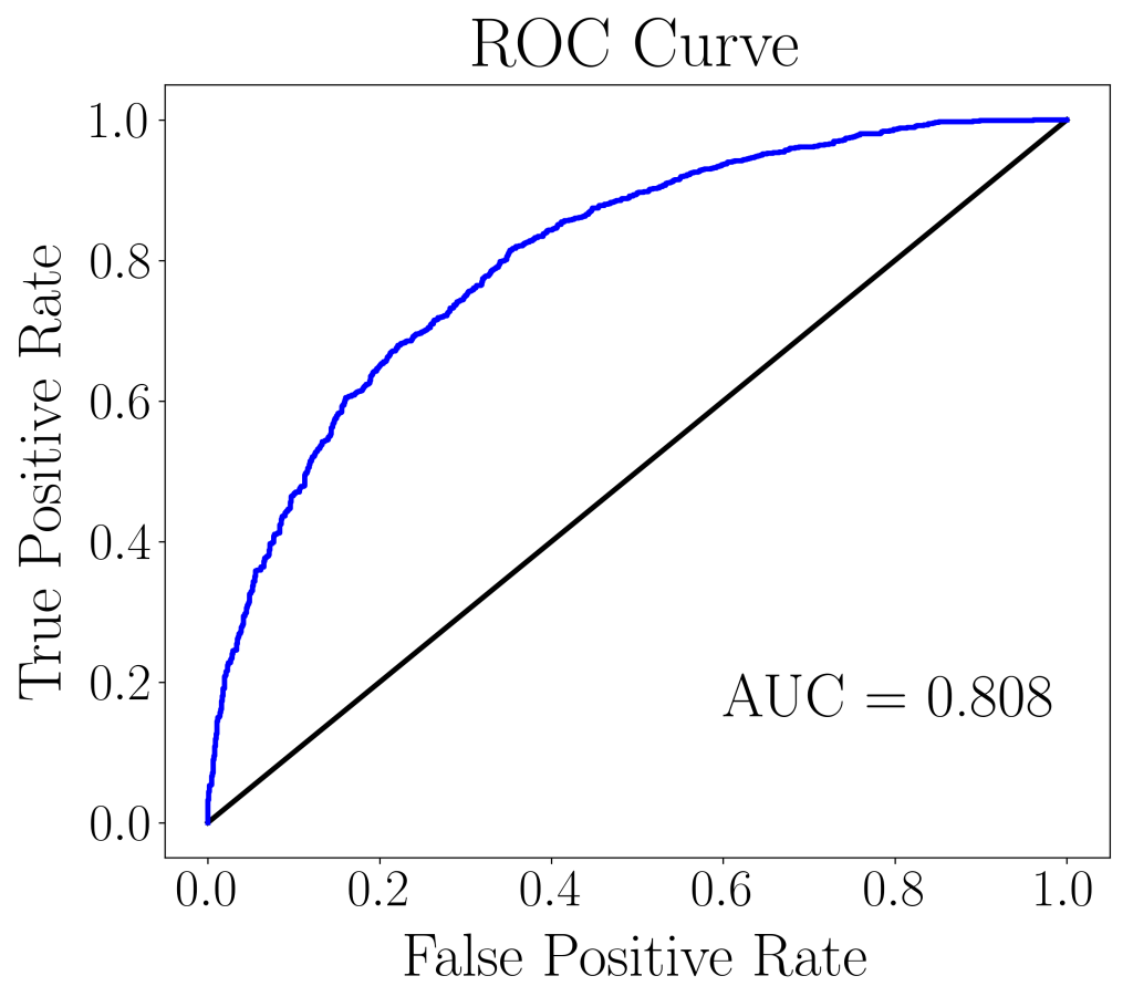
We validate the Machine Learning model by testing it against the validation set. The predicted outcomes are then compared with the actual outcomes, and we can further retrieve data such as probabilities, false positive rates, and true positive rates for plotting the ROC curve.
def predict_validation(model, X_test, y_test):
    from sklearn.metrics import roc_curve

    # Predict test set labels
    y_pred = model.predict(X_test)

    # Retrieve probability for ROC curve
    y_pred_prob = model.predict_proba(X_test)[:,1]

    # Output probability results
    pd.DataFrame(y_pred_prob.T).to_csv('csv/rf-prob.csv', index=False, header=False)

    fpr, tpr, thresholds = roc_curve(y_test, y_pred_prob)
    return fpr, tpr, y_pred, y_pred_prob
The ROC curve below can be plotted using the true positive rates against the false positive rates. In this case, the AUC (area under curve) score is 0.808, which is fairly decent considering that no hyperparameter tuning was done.
We can go further to plot feature importances, so that we can figure out what words have the most predictive power for deciding whether a movie review is negative (0) or positive (1).
importances_rf = pd.Series(model.feature_importances_, index=df.columns[:-1])
sorted_importances_rf = importances_rf.sort_values()[-10:]
sorted_importances_rf.plot(kind='barh', color='red')
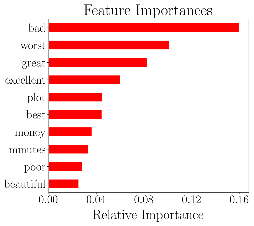
We see that words like ‘bad’, ‘great’, ‘worst’, and ‘excellent’ have the highest predictive power. And this makes total sense, considering that such words do convey the sentiment of strong opinions.
To further quantify the accuracy, we can also check the accuracy score between the train and test set.
# Evaluate test set accuracy
print('Accuracy score (train set) = %0.4f'%accuracy_score(y_train, model.predict(X_train)))
print('Accuracy score (test set) = %0.4f'%accuracy_score(y_test, y_pred))
The resulting accuracy score (train set) = 0.7684 and accuracy score (test set) = 0.7255. The two are approximately within the same order and we can say that our model is well-fitted. In the case where the score for the test set is a lot lower than the train set, the model has over-fitted and will not generalize well to other independent datasets.
We hope that you’ve enjoyed this article and can now add sentiment analysis to your bag of tricks as a data scientist!
